1 introduction
按照karpathy的教程,一步步的完成transformer的构建,并在这个过程中,加深对transformer设计的理解。
karpathy推荐在进行网络设计的过程中,同时利用jupyter notebook进行快速测试和python进行主要的网络的构建。
2 网络实现
2.1 数据的构建
- 读取text
text = open("input.txt", "r", encoding='utf-8').read()
words = sorted(set(''.join(text)))
vocab_size = len(words)
print(f'vocab_size is: {vocab_size}')
print(''.join(words))
print(text[:1000])
vocab_size is: 65
!$&',-.3:;?ABCDEFGHIJKLMNOPQRSTUVWXYZabcdefghijklmnopqrstuvwxyz
First Citizen:
Before we proceed any further, hear me speak.
All:
Speak, speak.
First Citizen:
You are all resolved rather to die than to famish?
- 将字符转换成数字
stoi = {ch : i for i, ch in enumerate(words)}
itos = {i : ch for i, ch in enumerate(words)}encode = lambda s: [stoi[ch] for ch in s]
decode = lambda l: ''.join([itos[i] for i in l])
print(encode("hii"))
print(decode(encode("hii")))
[46, 47, 47]
hii
- 制作数据集
import torch
# 生成数据集
data = torch.tensor(encode(text), dtype=torch.long)
print(len(data))
n = int(len(data) * 0.9)
train_data = data[:n]
val_data = data[n:]
print(train_data[:1000])
1115394
tensor([18, 47, 56, 57, 58, 1, 15, 47, 58, 47, 64, 43, 52, 10, 0, 14, 43, 44,
53, 56, 43, 1, 61, 43, 1, 54, 56, 53, 41, 43, 43, 42, 1, 39, 52, 63,
1, 44, 59, 56, 58, 46, 43, 56, 6, 1, 46, 43, 39, 56, 1, 51, 43, 1,
57, 54, 43, 39, 49, 8, 0, 0, 13, 50, 50, 10, 0, 31, 54, 43, 39, 49,
- 构建dataloader
import torch
batch_size = 4
torch.manual_seed(1337)
def get_batch(split):datasets = {'train': train_data,'val': val_data,}[split]ix = torch.randint(0, len(datasets) - block_size, (batch_size,))x = torch.stack([datasets[i:i+block_size] for i in ix])y = torch.stack([datasets[1+i:i+block_size+1] for i in ix])return x, yxb, yb = get_batch('train')
print(f'x shape is: {xb.shape}, y shape is: {yb.shape}')
print(f'x is {xb}')
print(f'y is {yb}')
x shape is: torch.Size([4, 8]), y shape is: torch.Size([4, 8])
x is tensor([[24, 43, 58, 5, 57, 1, 46, 43],
[44, 53, 56, 1, 58, 46, 39, 58],
[52, 58, 1, 58, 46, 39, 58, 1],
[25, 17, 27, 10, 0, 21, 1, 54]])
y is tensor([[43, 58, 5, 57, 1, 46, 43, 39],
[53, 56, 1, 58, 46, 39, 58, 1],
[58, 1, 58, 46, 39, 58, 1, 46],
[17, 27, 10, 0, 21, 1, 54, 39]])
2.2 构建pipeline
- 定义一个最简单的网络
import torch.nn as nn
import torch.nn.functional as F
torch.manual_seed(1337)
class BigramLanguageModel(nn.Module):def __init__(self, vocab_size):super().__init__()self.token_embedding_table = nn.Embedding(vocab_size, vocab_size)def forward(self, idx, targets=None):self.out = self.token_embedding_table(idx)return self.outxb, yb = get_batch('train')
model = BigramLanguageModel(vocab_size)
out = model(xb)
print(f'x shape is: {xb.shape}')
print(f'out shape is: {out.shape}')
x shape is: torch.Size([4, 8])
out shape is: torch.Size([4, 8, 65])
- 包含输出以后的完整的pipeline是
from typing import Iterator
import torch.nn as nn
import torch.nn.functional as F
torch.manual_seed(1337)
class BigramLanguageModel(nn.Module):def __init__(self, vocab_size):super().__init__()self.token_embedding_table = nn.Embedding(vocab_size, vocab_size)def forward(self, idx, targets=None):logits = self.token_embedding_table(idx)  # B, T, Cif targets is None:loss = Noneelse:B, T, C = logits.shapelogits = logits.view(B*T, C) # 这是很好理解的targets = targets.view(B*T) # 但是targets是B,Tloss = F.cross_entropy(logits, targets)return logits, lossdef generate(self, idx, max_new_tokens):for _ in range(max_new_tokens):logits, loss = self(idx)    logits = logits[:, -1, :]  # B, C    prob = F.softmax(logits, dim=-1)  # 对最后一维进行softmaxix = torch.multinomial(prob, num_samples=1) # B, Cprint(idx)idx = torch.cat((idx, ix), dim=1)   # B,T+1print(idx)return idx# ix = ix.view(B)xb, yb = get_batch('train')
model = BigramLanguageModel(vocab_size)
out, loss = model(xb)
print(f'x shape is: {xb.shape}')
print(f'out shape is: {out.shape}')idx = idx = torch.zeros((1, 1), dtype=torch.long)
print(decode(model.generate(idx, max_new_tokens=10)[0].tolist()))
# print(f'idx is {idx}')
x shape is: torch.Size([4, 8])
out shape is: torch.Size([4, 8, 65])
tensor([[0]])
tensor([[ 0, 50]])
tensor([[ 0, 50]])
tensor([[ 0, 50, 7]])
tensor([[ 0, 50, 7]])
tensor([[ 0, 50, 7, 29]])
tensor([[ 0, 50, 7, 29]])
tensor([[ 0, 50, 7, 29, 37]])
tensor([[ 0, 50, 7, 29, 37]])
tensor([[ 0, 50, 7, 29, 37, 48]])
tensor([[ 0, 50, 7, 29, 37, 48]])
tensor([[ 0, 50, 7, 29, 37, 48, 58]])
tensor([[ 0, 50, 7, 29, 37, 48, 58]])
tensor([[ 0, 50, 7, 29, 37, 48, 58, 5]])
tensor([[ 0, 50, 7, 29, 37, 48, 58, 5]])
tensor([[ 0, 50, 7, 29, 37, 48, 58, 5, 15]])
tensor([[ 0, 50, 7, 29, 37, 48, 58, 5, 15]])
tensor([[ 0, 50, 7, 29, 37, 48, 58, 5, 15, 24]])
tensor([[ 0, 50, 7, 29, 37, 48, 58, 5, 15, 24]])
tensor([[ 0, 50, 7, 29, 37, 48, 58, 5, 15, 24, 12]])
l-QYjt’CL?
这里有几个地方需要注意,首先输入输出是:
x is tensor([[24, 43, 58, 5, 57, 1, 46, 43],
[44, 53, 56, 1, 58, 46, 39, 58],
[52, 58, 1, 58, 46, 39, 58, 1],
[25, 17, 27, 10, 0, 21, 1, 54]])
y is tensor([[43, 58, 5, 57, 1, 46, 43, 39],
[53, 56, 1, 58, 46, 39, 58, 1],
[58, 1, 58, 46, 39, 58, 1, 46],
[17, 27, 10, 0, 21, 1, 54, 39]])
并且这个pipeline,网络对输入的长度也没有限制
- 开始训练
这个时候我们需要构建一个完整的训练代码,如果还是用jupyter notebook,每次改变了网络的一个组成部分,需要重新执行很多地方,比较麻烦,所以构建一个.py文件。
import torch
import torch.nn as nn
import torch.nn.functional as F# hyperparameters
batch_size = 32
block_size = 8
max_iter = 3000
eval_interval = 300
learning_rate = 1e-2
device = 'cuda' if torch.cuda.is_available() else 'cpu'
eval_iters = 200
# ---------------------torch.manual_seed(1337)text = open("input.txt", "r", encoding='utf-8').read()
chars = sorted(list(set(text)))
vocab_size = len(chars)stoi = {ch : i for i, ch in enumerate(chars)}
itos = {i : ch for i, ch in enumerate(chars)}
encode = lambda s: [stoi[ch] for ch in s]
decode = lambda l: ''.join([itos[i] for i in l])# 生成数据集
data = torch.tensor(encode(text), dtype=torch.long)
n = int(len(data) * 0.9)
train_data = data[:n]
val_data = data[n:]def get_batch(split):datasets = {'train': train_data,'val': val_data,}[split]ix = torch.randint(0, len(datasets) - block_size, (batch_size,))x = torch.stack([datasets[i:i+block_size] for i in ix])y = torch.stack([datasets[1+i:i+block_size+1] for i in ix])x, y = x.to(device), y.to(device)return x, y@torch.no_grad()
def estimate_loss():out = {}model.eval()for split in ['train', 'val']:losses = torch.zeros(eval_iters)for k in range(eval_iters):X, Y = get_batch(split)logits, loss = model(X, Y)losses[k] = loss.item()out[split] = losses.mean()model.train()return outclass BigramLanguageModel(nn.Module):def __init__(self, vocab_size):super().__init__()self.token_embedding_table = nn.Embedding(vocab_size, vocab_size)def forward(self, idx, targets=None):# import pdb; pdb.set_trace()logits = self.token_embedding_table(idx)  # B, T, Cif targets is None:loss = Noneelse:B, T, C = logits.shapelogits = logits.view(B*T, C) # 这是很好理解的targets = targets.view(B*T) # 但是targets是B,T, C其实并不好理解loss = F.cross_entropy(logits, targets)return logits, lossdef generate(self, idx, max_new_tokens):for _ in range(max_new_tokens):logits, loss = self(idx)    logits = logits[:, -1, :]  # B, C    prob = F.softmax(logits, dim=-1)  # 对最后一维进行softmaxix = torch.multinomial(prob, num_samples=1) # B, 1# print(idx)idx = torch.cat((idx, ix), dim=1)   # B,T+1# print(idx)return idxmodel = BigramLanguageModel(vocab_size)
m = model.to(device)
optimizer = torch.optim.AdamW(model.parameters(), lr=learning_rate)lossi = []
for iter in range(max_iter):if iter % eval_interval == 0:losses = estimate_loss()print(f'step {iter}: train loss {losses["train"]:.4f}, val loss {losses["val"]:.4f}')xb, yb = get_batch('train')out, loss = m(xb, yb)optimizer.zero_grad(set_to_none=True)loss.backward()optimizer.step()# generate from the model
context = torch.zeros((1,1), dtype=torch.long, device=device)
print(decode(m.generate(context, max_new_tokens=500)[0].tolist()))
输出的结果是
step 0: train loss 4.7305, val loss 4.7241
step 300: train loss 2.8110, val loss 2.8249
step 600: train loss 2.5434, val loss 2.5682
step 900: train loss 2.4932, val loss 2.5088
step 1200: train loss 2.4863, val loss 2.5035
step 1500: train loss 2.4665, val loss 2.4921
step 1800: train loss 2.4683, val loss 2.4936
step 2100: train loss 2.4696, val loss 2.4846
step 2400: train loss 2.4638, val loss 2.4879
step 2700: train loss 2.4738, val loss 2.4911
CEThik brid owindakis b, bth
HAPet bobe d e.
S:
O:3 my d?
LUCous:
Wanthar u qur, t.
War dXENDoate awice my.
Hastarom oroup
Yowhthetof isth ble mil ndill, ath iree sengmin lat Heriliovets, and Win nghir.
Swanousel lind me l.
HAshe ce hiry:
Supr aisspllw y.
Hentofu n Boopetelaves
MPOLI s, d mothakleo Windo whth eisbyo the m dourive we higend t so mower; te
AN ad nterupt f s ar igr t m:
Thin maleronth,
Mad
RD:
WISo myrangoube!
KENob&y, wardsal thes ghesthinin couk ay aney IOUSts I&fr y ce.
J
2.3 self-attention
我们处理当前的字符的时候,需要和历史字符进行通信,历史字符可以看成是某一种特征,使用最简单的均值提取的方式提取历史字符的feature
# 最简单的通信方式,将当前的字符和之前的字符平均进行沟通
# 可以看成是history information的features
a = torch.tril(torch.ones(3, 3))
print(a)
a = torch.tril(a) / torch.sum(a, 1, keepdim=True)
print(a)
tensor([[1., 0., 0.],
[1., 1., 0.],
[1., 1., 1.]])
tensor([[1.0000, 0.0000, 0.0000],
[0.5000, 0.5000, 0.0000],
[0.3333, 0.3333, 0.3333]])
可以采用softmax的方式进行mask
import torch.nn.functional as F
tril = torch.tril(torch.ones(T, T))  # 某种意义上的Q
wei = torch.zeros(T, T) # K
wei = wei.masked_fill(tril == 0, float('-inf'))
print(wei)
wei = F.softmax(wei)
print(wei)
tensor([[0., -inf, -inf, -inf, -inf, -inf, -inf, -inf],
[0., 0., -inf, -inf, -inf, -inf, -inf, -inf],
[0., 0., 0., -inf, -inf, -inf, -inf, -inf],
[0., 0., 0., 0., -inf, -inf, -inf, -inf],
[0., 0., 0., 0., 0., -inf, -inf, -inf],
[0., 0., 0., 0., 0., 0., -inf, -inf],
[0., 0., 0., 0., 0., 0., 0., -inf],
[0., 0., 0., 0., 0., 0., 0., 0.]])
tensor([[1.0000, 0.0000, 0.0000, 0.0000, 0.0000, 0.0000, 0.0000, 0.0000],
[0.5000, 0.5000, 0.0000, 0.0000, 0.0000, 0.0000, 0.0000, 0.0000],
[0.3333, 0.3333, 0.3333, 0.0000, 0.0000, 0.0000, 0.0000, 0.0000],
[0.2500, 0.2500, 0.2500, 0.2500, 0.0000, 0.0000, 0.0000, 0.0000],
[0.2000, 0.2000, 0.2000, 0.2000, 0.2000, 0.0000, 0.0000, 0.0000],
[0.1667, 0.1667, 0.1667, 0.1667, 0.1667, 0.1667, 0.0000, 0.0000],
[0.1429, 0.1429, 0.1429, 0.1429, 0.1429, 0.1429, 0.1429, 0.0000],
[0.1250, 0.1250, 0.1250, 0.1250, 0.1250, 0.1250, 0.1250, 0.1250]])
特征提取的结果
xbow2 = wei @ x # (T, T) @ (B, T, C) --> (B, T, C)  # x对应v
print(xbow2.shape)
torch.Size([4, 8, 2])
加上pos_emb现在的forward版本
def forward(self, idx, targets=None):# import pdb; pdb.set_trace()tok_emb = self.token_embedding_table(idx) # B, T, C(n_emb)pos_emb = self.position_embedding_table(torch.range(T, device=device)) # T,C # positional encodingx = tok_emb + pos_emb # (B, T, C) broadcastinglogits = self.lm_head(x) # B, T, C(vocab_size)if targets is None:loss = Noneelse:B, T, C = logits.shapelogits = logits.view(B*T, C) # 这是很好理解的targets = targets.view(B*T) # 但是targets是B,T, C其实并不好理解loss = F.cross_entropy(logits, targets)return logits, loss
karpathy 给出的一些启示
- Attention is a communication mechanism. Can be seen as nodes in a directed graph looking at each other and aggregating information with a weighted sum from all nodes that point to them, with data-dependent weights.
- There is no notion of space. Attention simply acts over a set of vectors. This is why we need to positionally encode tokens.
- Each example across batch dimension is of course processed completely independently and never “talk” to each other
- In an “encoder” attention block just delete the single line that does masking with tril, allowing all tokens to communicate. This block here is called a “decoder” attention block because it has triangular masking, and is usually used in autoregressive settings, like language modeling.
- “self-attention” just means that the keys and values are produced from the same source as queries. In “cross-attention”, the queries still get produced from x, but the keys and values come from some other, external source (e.g. an encoder module)
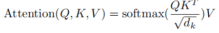
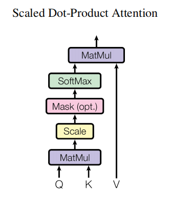
- “Scaled” attention additional divides wei by 1/sqrt(head_size). This makes it so when input Q,K are unit variance, wei will be unit variance too and Softmax will stay diffuse and not saturate too much. Illustration below
attention的公式其中scale是为了保证两个分布相乘的时候,方差不变的。
k = torch.randn(B, T, head_size)
q = torch.randn(B, T, head_size)
wei = q @ k.transpose(-2, -1)
wei_scale = wei / head_size**0.5
print(k.var())
print(q.var())
print(wei.var())
print(wei_scale.var())
输出结果
tensor(1.0278)
tensor(0.9802)
tensor(15.9041)
tensor(0.9940)
初始化对结果的影响很大,实际上来说我们还是很希望softmax初始化的结果是一个方差较小的分布,如果不进行scale
torch.softmax(torch.tensor([0.1, -0.2, 0.3, -0.2, 0.5]) * 8, dim=-1)
tensor([0.0326, 0.0030, 0.1615, 0.0030, 0.8000])
对原来的py文件做一些修改:
class Head(nn.Module):def __init__(self, head_size):super().__init__()self.query = nn.Linear(n_embd, head_size, bias=False)self.key = nn.Linear(n_embd, head_size, bias=False)self.value = nn.Linear(n_embd, head_size, bias=False)self.register_buffer('tril', torch.tril(torch.ones(block_size, block_size)))def forward(self, x):# import pdb; pdb.set_trace()B, T, C = x.shape q = self.query(x) #(B, T, C)k = self.key(x) #(B, T, C)v = self.value(x) #(B, T, C)wei = q @ k.transpose(-2, -1) * C**-0.5 # (B,T,C)@(B,C,T) --> (B, T, T)wei = wei.masked_fill(self.tril[:T, :T] == 0, float('-inf')) wei = F.softmax(wei, dim=-1) # (B, T, T)out = wei @ v #(B, T, T) @ (B, T, C) --> (B, T, C)return out
修改模型
class BigramLanguageModel(nn.Module):def __init__(self, vocab_size):super().__init__()self.token_embedding_table = nn.Embedding(vocab_size, n_embd)self.position_embedding_table = nn.Embedding(block_size, n_embd)self.sa_head = Head(n_embd) # head的尺寸保持不变self.lm_head = nn.Linear(n_embd, vocab_size)def forward(self, idx, targets=None):# import pdb; pdb.set_trace()B, T = idx.shapetok_emb = self.token_embedding_table(idx) # B, T, C(n_emb)pos_emb = self.position_embedding_table(torch.arange(T, device=device)) # T,C # positional encodingx = tok_emb + pos_emb # (B, T, C) broadcastingx = self.sa_head(x)logits = self.lm_head(x) # B, T, C(vocab_size)if targets is None:loss = Noneelse:B, T, C = logits.shapelogits = logits.view(B*T, C) # 这是很好理解的targets = targets.view(B*T) # 但是targets是B,T, C其实并不好理解loss = F.cross_entropy(logits, targets)return logits, lossdef generate(self, idx, max_new_tokens):for _ in range(max_new_tokens):idx_cmd = idx[:, -block_size:] # (B, T)logits, loss = self(idx_cmd) logits = logits[:, -1, :] # B, C prob = F.softmax(logits, dim=-1) # 对最后一维进行softmaxix = torch.multinomial(prob, num_samples=1) # B, 1# print(idx)idx = torch.cat((idx, ix), dim=1) # B,T+1# print(idx)return idx
加上self-attention的结果
step 4500: train loss 2.3976, val loss 2.4041
2.4 multi-head attention
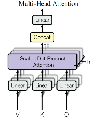
这里借鉴了group convolutional 的思想,
class MultiHeadAttention(nn.Module):""" multiple head of self attention in parallel """def __init__(self, num_heads, head_size):super().__init__()self.heads = nn.ModuleList([Head(head_size) for _ in range(num_heads)])def forward(self, x):return torch.cat([h(x) for h in self.heads], dim=-1)
应用的时候
self.sa_head = MultiHeadAttention(4, n_embd//4) # head的尺寸保持不变
训练的结果
step 4500: train loss 2.2679, val loss 2.2789
2.5 feedforward network
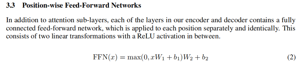
加上feedforward的结果
step 4500: train loss 2.2337, val loss 2.2476
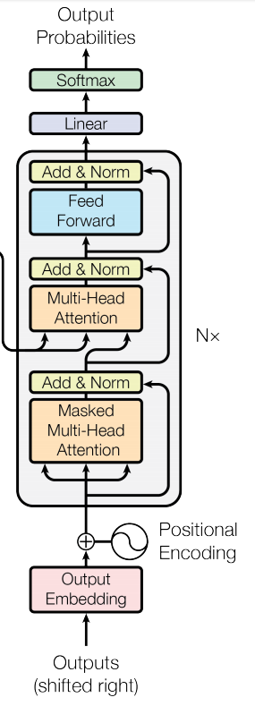
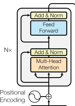
同时用一个block表示这个这个单元,
一个transform的block可以理解成一个connection 组成部分+computation组成部分
class Block(nn.Module):def __init__(self, n_embd, n_head):super().__init__()head_size = n_embd // n_headself.sa = MultiHeadAttention(n_head, head_size)self.ffwd = FeedForward(n_embd)def forward(self, x):x = self.sa(x)x = self.ffwd(x)return x
修改模型的定义
class BigramLanguageModel(nn.Module):def __init__(self, vocab_size):super().__init__()self.token_embedding_table = nn.Embedding(vocab_size, n_embd)self.position_embedding_table = nn.Embedding(block_size, n_embd)self.blocks = nn.Sequential(Block(n_embd, n_head=4),Block(n_embd, n_head=4),Block(n_embd, n_head=4),)self.lm_head = nn.Linear(n_embd, vocab_size)def forward(self, idx, targets=None):# import pdb; pdb.set_trace()B, T = idx.shapetok_emb = self.token_embedding_table(idx) # B, T, C(n_emb)pos_emb = self.position_embedding_table(torch.arange(T, device=device)) # T,C # positional encodingx = tok_emb + pos_emb # (B, T, C) broadcastingx = self.blocks(x)logits = self.lm_head(x) # B, T, C(vocab_size)if targets is None:loss = Noneelse:B, T, C = logits.shapelogits = logits.view(B*T, C) # 这是很好理解的targets = targets.view(B*T) # 但是targets是B,T, C其实并不好理解loss = F.cross_entropy(logits, targets)return logits, loss
2.6 Residual network
现在模型的深度已经很深了,直接训练很可能无法很好的收敛,需要另外一个很重要的工具,残差网络。
class Block(nn.Module):def __init__(self, n_embd, n_head):super().__init__()head_size = n_embd // n_headself.sa = MultiHeadAttention(n_head, head_size)self.ffwd = FeedForward(n_embd)def forward(self, x):x = x + self.sa(x)x = x + self.ffwd(x)return x
深度扩充了以后,很容易过拟合了
step 4500: train loss 2.0031, val loss 2.1067
2.7 Layer normalization
我们先来看一下很基础的batchnorm。加入x,y 是两个独立,并且均值为0,方差为1的分布。
根据Var(xy)=E(X)^2 * Var(Y) + E(Y)^2 * Var(X) + Var(X) * Var(Y)=1
再来看矩阵相乘后,每一行变成了T2个独立同分布的乘积,根据中心极限定理:它们的和将近似服从正态分布,均值为各随机变量均值之和,方差为各随机变量方差之和。
也就是说矩阵相乘后的第一列的var=T2*1, mean=0
所以在矩阵相乘的时候,进行scale T 2 \sqrt{T2} T2 可以normalize(var 是平方,所以用了开根号)

x = torch.ones(5,5)
x = torch.tril(x)
print(x)
print(x.mean(dim=0))
print(x.mean(dim=1))
观察一下矩阵normalize的特点
tensor([[1., 0., 0., 0., 0.],
[1., 1., 0., 0., 0.],
[1., 1., 1., 0., 0.],
[1., 1., 1., 1., 0.],
[1., 1., 1., 1., 1.]])
tensor([1.0000, 0.8000, 0.6000, 0.4000, 0.2000])
tensor([0.2000, 0.4000, 0.6000, 0.8000, 1.0000])
class BatchNorm1d:def __init__(self, dim, eps=1e-5, momentum=0.1):self.eps = epsself.momentum = momentumself.training = True# parameters (trained with backprop)self.gamma = torch.ones(dim)self.beta = torch.zeros(dim)# buffers (trained with a running 'momentum update')self.running_mean = torch.zeros(dim)self.running_var = torch.ones(dim)def __call__(self, x):# calculate the forward passif self.training:if x.ndim == 2:dim = 0elif x.ndim == 3:dim = (0,1)xmean = x.mean(dim, keepdim=True) # batch meanxvar = x.var(dim, keepdim=True) # batch varianceelse:xmean = self.running_meanxvar = self.running_varxhat = (x - xmean) / torch.sqrt(xvar + self.eps) # normalize to unit varianceself.out = self.gamma * xhat + self.beta# update the buffersif self.training:with torch.no_grad():self.running_mean = (1 - self.momentum) * self.running_mean + self.momentum * xmeanself.running_var = (1 - self.momentum) * self.running_var + self.momentum * xvarreturn self.outdef parameters(self):return [self.gamma, self.beta]
BatchNormalized对一列进行normalized, layernormalize 对一行进行normalized。
class BatchNorm1d:def __init__(self, dim, eps=1e-5, momentum=0.1):self.eps = epsself.momentum = momentumself.training = True# parameters (trained with backprop)self.gamma = torch.ones(dim)self.beta = torch.zeros(dim)# buffers (trained with a running 'momentum update')self.running_mean = torch.zeros(dim)self.running_var = torch.ones(dim)def __call__(self, x):# calculate the forward passif self.training:dim = 1xmean = x.mean(dim, keepdim=True) # batch meanxvar = x.var(dim, keepdim=True) # batch varianceelse:xmean = self.running_meanxvar = self.running_varxhat = (x - xmean) / torch.sqrt(xvar + self.eps) # normalize to unit varianceself.out = self.gamma * xhat + self.beta# update the buffersif self.training:with torch.no_grad():self.running_mean = (1 - self.momentum) * self.running_mean + self.momentum * xmeanself.running_var = (1 - self.momentum) * self.running_var + self.momentum * xvarreturn self.outdef parameters(self):return [self.gamma, self.beta]
如今用的比较 的模式
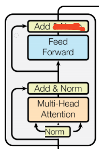
对应的代码
``python
class Block(nn.Module):
def init(self, n_embd, n_head):
super().init()
head_size = n_embd // n_head
self.sa = MultiHeadAttention(n_head, head_size)
self.ffwd = FeedForward(n_embd)
self.ln1 = nn.LayerNorm(n_embd)
self.ln2 = nn.LayerNorm(n_embd)
def forward(self, x):x = x + self.sa(self.ln1(x))x = x + self.ffwd(self.ln2(x))return x
并且一般会在连续的decoder block 模块后添加一个layerNorm
```python
class BigramLanguageModel(nn.Module):def __init__(self, vocab_size):super().__init__()self.token_embedding_table = nn.Embedding(vocab_size, n_embd)self.position_embedding_table = nn.Embedding(block_size, n_embd)self.blocks = nn.Sequential(Block(n_embd, n_head=4),Block(n_embd, n_head=4),Block(n_embd, n_head=4),nn.LayerNorm(n_embd),)self.lm_head = nn.Linear(n_embd, vocab_size)
加上layerNormlization以后,精度又上升了一些
step 4500: train loss 1.9931, val loss 2.0892
现在训练误差和验证误差的loss比较大 ,需要想办法解决一下。
2.8 使用dropout
- 在head 使用dropout,防止模型被特定的feature给过分影响了提高模型的鲁棒性。
def forward(self, x):# import pdb; pdb.set_trace()B, T, C = x.shape q = self.query(x) #(B, T, C)k = self.key(x) #(B, T, C)v = self.value(x) #(B, T, C)wei = q @ k.transpose(-2, -1) * C**-0.5 # (B,T,C)@(B,C,T) --> (B, T, T)wei = wei.masked_fill(self.tril[:T, :T] == 0, float('-inf')) wei = F.softmax(wei, dim=-1) # (B, T, T)wei = self.dropout(wei)out = wei @ v #(B, T, T) @ (B, T, C) --> (B, T, C)return out
- 在multihead上使用dropout,也是同样的原理,防止特定feature过分影响了模型
def forward(self, x):out = torch.cat([h(x) for h in self.heads], dim=-1)out = self.dropout(self.proj(out))return out
- 在计算单元的输出结果前使用dropout
class FeedForward(nn.Module):def __init__(self, n_embd):super().__init__()self.net = nn.Sequential(nn.Linear(n_embd, 4 * n_embd),nn.ReLU(),nn.Linear(4 * n_embd, n_embd),nn.Dropout(dropout),)
修改设定参数
# hyperparameters
batch_size = 64
block_size = 256
max_iter = 5000
eval_interval = 500
learning_rate = 3e-4    # self-attention can't tolerate very high learnning rate
device = 'cuda' if torch.cuda.is_available() else 'cpu'
eval_iters = 200
n_embd = 384
n_layer = 6
n_head = 6
dropout = 0.2
step 4500: train loss 1.1112, val loss 1.4791
References
[1] https://www.youtube.com/watch?v=kCc8FmEb1nY