Pandas 2.2 中文官方教程和指南（二十五·二）

新列

使用 DataFrame.map（以前称为 applymap）高效动态创建新列

In [53]: df = pd.DataFrame({"AAA": [1, 2, 1, 3], "BBB": [1, 1, 2, 2], "CCC": [2, 1, 3, 1]})In [54]: df
Out[54]: AAA  BBB  CCC
0    1    1    2
1    2    1    1
2    1    2    3
3    3    2    1In [55]: source_cols = df.columns  # Or some subset would work tooIn [56]: new_cols = [str(x) + "_cat" for x in source_cols]In [57]: categories = {1: "Alpha", 2: "Beta", 3: "Charlie"}In [58]: df[new_cols] = df[source_cols].map(categories.get)In [59]: df
Out[59]: AAA  BBB  CCC  AAA_cat BBB_cat  CCC_cat
0    1    1    2    Alpha   Alpha     Beta
1    2    1    1     Beta   Alpha    Alpha
2    1    2    3    Alpha    Beta  Charlie
3    3    2    1  Charlie    Beta    Alpha

在 groupby 中使用 min() 时保留其他列

In [60]: df = pd.DataFrame(....:    {"AAA": [1, 1, 1, 2, 2, 2, 3, 3], "BBB": [2, 1, 3, 4, 5, 1, 2, 3]}....: )....: In [61]: df
Out[61]: AAA  BBB
0    1    2
1    1    1
2    1    3
3    2    4
4    2    5
5    2    1
6    3    2
7    3    3

方法 1：使用 idxmin() 获取最小值的索引

In [62]: df.loc[df.groupby("AAA")["BBB"].idxmin()]
Out[62]: AAA  BBB
1    1    1
5    2    1
6    3    2

方法 2：排序然后取每个的第一个

In [63]: df.sort_values(by="BBB").groupby("AAA", as_index=False).first()
Out[63]: AAA  BBB
0    1    1
1    2    1
2    3    2

注意相同的结果，除了索引。

多重索引

多级索引文档。

从带标签的框架创建 MultiIndex

In [64]: df = pd.DataFrame(....:    {....:        "row": [0, 1, 2],....:        "One_X": [1.1, 1.1, 1.1],....:        "One_Y": [1.2, 1.2, 1.2],....:        "Two_X": [1.11, 1.11, 1.11],....:        "Two_Y": [1.22, 1.22, 1.22],....:    }....: )....: In [65]: df
Out[65]: row  One_X  One_Y  Two_X  Two_Y
0    0    1.1    1.2   1.11   1.22
1    1    1.1    1.2   1.11   1.22
2    2    1.1    1.2   1.11   1.22# As Labelled Index
In [66]: df = df.set_index("row")In [67]: df
Out[67]: One_X  One_Y  Two_X  Two_Y
row 
0      1.1    1.2   1.11   1.22
1      1.1    1.2   1.11   1.22
2      1.1    1.2   1.11   1.22# With Hierarchical Columns
In [68]: df.columns = pd.MultiIndex.from_tuples([tuple(c.split("_")) for c in df.columns])In [69]: df
Out[69]: One        Two X    Y     X     Y
row 
0    1.1  1.2  1.11  1.22
1    1.1  1.2  1.11  1.22
2    1.1  1.2  1.11  1.22# Now stack & Reset
In [70]: df = df.stack(0, future_stack=True).reset_index(1)In [71]: df
Out[71]: level_1     X     Y
row 
0       One  1.10  1.20
0       Two  1.11  1.22
1       One  1.10  1.20
1       Two  1.11  1.22
2       One  1.10  1.20
2       Two  1.11  1.22# And fix the labels (Notice the label 'level_1' got added automatically)
In [72]: df.columns = ["Sample", "All_X", "All_Y"]In [73]: df
Out[73]: Sample  All_X  All_Y
row 
0      One   1.10   1.20
0      Two   1.11   1.22
1      One   1.10   1.20
1      Two   1.11   1.22
2      One   1.10   1.20
2      Two   1.11   1.22

算术

对需要广播的 MultiIndex 执行算术运算

In [74]: cols = pd.MultiIndex.from_tuples(....:    [(x, y) for x in ["A", "B", "C"] for y in ["O", "I"]]....: )....: In [75]: df = pd.DataFrame(np.random.randn(2, 6), index=["n", "m"], columns=cols)In [76]: df
Out[76]: A                   B                   C O         I         O         I         O         I
n  0.469112 -0.282863 -1.509059 -1.135632  1.212112 -0.173215
m  0.119209 -1.044236 -0.861849 -2.104569 -0.494929  1.071804In [77]: df = df.div(df["C"], level=1)In [78]: df
Out[78]: A                   B              C O         I         O         I    O    I
n  0.387021  1.633022 -1.244983  6.556214  1.0  1.0
m -0.240860 -0.974279  1.741358 -1.963577  1.0  1.0

切片

使用 xs 切片 MultiIndex

In [79]: coords = [("AA", "one"), ("AA", "six"), ("BB", "one"), ("BB", "two"), ("BB", "six")]In [80]: index = pd.MultiIndex.from_tuples(coords)In [81]: df = pd.DataFrame([11, 22, 33, 44, 55], index, ["MyData"])In [82]: df
Out[82]: MyData
AA one      11six      22
BB one      33two      44six      55

要获取索引的第一级和第一轴的交叉部分：

# Note : level and axis are optional, and default to zero
In [83]: df.xs("BB", level=0, axis=0)
Out[83]: MyData
one      33
two      44
six      55

…现在是第一轴的第二级。

In [84]: df.xs("six", level=1, axis=0)
Out[84]: MyData
AA      22
BB      55

使用 xs 切片 MultiIndex，方法 #2

In [85]: import itertoolsIn [86]: index = list(itertools.product(["Ada", "Quinn", "Violet"], ["Comp", "Math", "Sci"]))In [87]: headr = list(itertools.product(["Exams", "Labs"], ["I", "II"]))In [88]: indx = pd.MultiIndex.from_tuples(index, names=["Student", "Course"])In [89]: cols = pd.MultiIndex.from_tuples(headr)  # Notice these are un-namedIn [90]: data = [[70 + x + y + (x * y) % 3 for x in range(4)] for y in range(9)]In [91]: df = pd.DataFrame(data, indx, cols)In [92]: df
Out[92]: Exams     Labs I  II    I  II
Student Course 
Ada     Comp      70  71   72  73Math      71  73   75  74Sci       72  75   75  75
Quinn   Comp      73  74   75  76Math      74  76   78  77Sci       75  78   78  78
Violet  Comp      76  77   78  79Math      77  79   81  80Sci       78  81   81  81In [93]: All = slice(None)In [94]: df.loc["Violet"]
Out[94]: Exams     Labs I  II    I  II
Course 
Comp      76  77   78  79
Math      77  79   81  80
Sci       78  81   81  81In [95]: df.loc[(All, "Math"), All]
Out[95]: Exams     Labs I  II    I  II
Student Course 
Ada     Math      71  73   75  74
Quinn   Math      74  76   78  77
Violet  Math      77  79   81  80In [96]: df.loc[(slice("Ada", "Quinn"), "Math"), All]
Out[96]: Exams     Labs I  II    I  II
Student Course 
Ada     Math      71  73   75  74
Quinn   Math      74  76   78  77In [97]: df.loc[(All, "Math"), ("Exams")]
Out[97]: I  II
Student Course 
Ada     Math    71  73
Quinn   Math    74  76
Violet  Math    77  79In [98]: df.loc[(All, "Math"), (All, "II")]
Out[98]: Exams LabsII   II
Student Course 
Ada     Math      73   74
Quinn   Math      76   77
Violet  Math      79   80

使用 xs 设置 MultiIndex 的部分

排序

按特定列或有序列的列排序，使用 MultiIndex

In [99]: df.sort_values(by=("Labs", "II"), ascending=False)
Out[99]: Exams     Labs I  II    I  II
Student Course 
Violet  Sci       78  81   81  81Math      77  79   81  80Comp      76  77   78  79
Quinn   Sci       75  78   78  78Math      74  76   78  77Comp      73  74   75  76
Ada     Sci       72  75   75  75Math      71  73   75  74Comp      70  71   72  73

部分选择，需要排序 GH 2995

层级

在 MultiIndex 前添加一个级别

展平分层列

算术

对需要广播的 MultiIndex 执行算术运算

In [74]: cols = pd.MultiIndex.from_tuples(....:    [(x, y) for x in ["A", "B", "C"] for y in ["O", "I"]]....: )....: In [75]: df = pd.DataFrame(np.random.randn(2, 6), index=["n", "m"], columns=cols)In [76]: df
Out[76]: A                   B                   C O         I         O         I         O         I
n  0.469112 -0.282863 -1.509059 -1.135632  1.212112 -0.173215
m  0.119209 -1.044236 -0.861849 -2.104569 -0.494929  1.071804In [77]: df = df.div(df["C"], level=1)In [78]: df
Out[78]: A                   B              C O         I         O         I    O    I
n  0.387021  1.633022 -1.244983  6.556214  1.0  1.0
m -0.240860 -0.974279  1.741358 -1.963577  1.0  1.0

切片

使用 xs 切片 MultiIndex

In [79]: coords = [("AA", "one"), ("AA", "six"), ("BB", "one"), ("BB", "two"), ("BB", "six")]In [80]: index = pd.MultiIndex.from_tuples(coords)In [81]: df = pd.DataFrame([11, 22, 33, 44, 55], index, ["MyData"])In [82]: df
Out[82]: MyData
AA one      11six      22
BB one      33two      44six      55

要获取索引的第一级和第一轴的交叉部分：

# Note : level and axis are optional, and default to zero
In [83]: df.xs("BB", level=0, axis=0)
Out[83]: MyData
one      33
two      44
six      55

…现在是第一轴的第二级。

In [84]: df.xs("six", level=1, axis=0)
Out[84]: MyData
AA      22
BB      55

使用 xs 切片 MultiIndex，方法 #2

In [85]: import itertoolsIn [86]: index = list(itertools.product(["Ada", "Quinn", "Violet"], ["Comp", "Math", "Sci"]))In [87]: headr = list(itertools.product(["Exams", "Labs"], ["I", "II"]))In [88]: indx = pd.MultiIndex.from_tuples(index, names=["Student", "Course"])In [89]: cols = pd.MultiIndex.from_tuples(headr)  # Notice these are un-namedIn [90]: data = [[70 + x + y + (x * y) % 3 for x in range(4)] for y in range(9)]In [91]: df = pd.DataFrame(data, indx, cols)In [92]: df
Out[92]: Exams     Labs I  II    I  II
Student Course 
Ada     Comp      70  71   72  73Math      71  73   75  74Sci       72  75   75  75
Quinn   Comp      73  74   75  76Math      74  76   78  77Sci       75  78   78  78
Violet  Comp      76  77   78  79Math      77  79   81  80Sci       78  81   81  81In [93]: All = slice(None)In [94]: df.loc["Violet"]
Out[94]: Exams     Labs I  II    I  II
Course 
Comp      76  77   78  79
Math      77  79   81  80
Sci       78  81   81  81In [95]: df.loc[(All, "Math"), All]
Out[95]: Exams     Labs I  II    I  II
Student Course 
Ada     Math      71  73   75  74
Quinn   Math      74  76   78  77
Violet  Math      77  79   81  80In [96]: df.loc[(slice("Ada", "Quinn"), "Math"), All]
Out[96]: Exams     Labs I  II    I  II
Student Course 
Ada     Math      71  73   75  74
Quinn   Math      74  76   78  77In [97]: df.loc[(All, "Math"), ("Exams")]
Out[97]: I  II
Student Course 
Ada     Math    71  73
Quinn   Math    74  76
Violet  Math    77  79In [98]: df.loc[(All, "Math"), (All, "II")]
Out[98]: Exams LabsII   II
Student Course 
Ada     Math      73   74
Quinn   Math      76   77
Violet  Math      79   80

使用 xs 设置 MultiIndex 的部分

排序

按特定列或有序列的列排序，使用 MultiIndex

In [99]: df.sort_values(by=("Labs", "II"), ascending=False)
Out[99]: Exams     Labs I  II    I  II
Student Course 
Violet  Sci       78  81   81  81Math      77  79   81  80Comp      76  77   78  79
Quinn   Sci       75  78   78  78Math      74  76   78  77Comp      73  74   75  76
Ada     Sci       72  75   75  75Math      71  73   75  74Comp      70  71   72  73

部分选择，需要排序 GH 2995

层级

在 MultiIndex 前添加一个级别

展平分层列

缺失数据

缺失数据文档。

填充反转时间序列

In [100]: df = pd.DataFrame(.....:    np.random.randn(6, 1),.....:    index=pd.date_range("2013-08-01", periods=6, freq="B"),.....:    columns=list("A"),.....: ).....: In [101]: df.loc[df.index[3], "A"] = np.nanIn [102]: df
Out[102]: A
2013-08-01  0.721555
2013-08-02 -0.706771
2013-08-05 -1.039575
2013-08-06       NaN
2013-08-07 -0.424972
2013-08-08  0.567020In [103]: df.bfill()
Out[103]: A
2013-08-01  0.721555
2013-08-02 -0.706771
2013-08-05 -1.039575
2013-08-06 -0.424972
2013-08-07 -0.424972
2013-08-08  0.567020

在 NaN 值处重置累积和

替换

使用带有 backrefs 的 replace

替换

使用带有 backrefs 的 replace

分组

分组文档。

应用基本分组

与 agg 不同，apply 的可调用函数传递一个子数据框，使您可以访问所有列

In [104]: df = pd.DataFrame(.....:    {.....:        "animal": "cat dog cat fish dog cat cat".split(),.....:        "size": list("SSMMMLL"),.....:        "weight": [8, 10, 11, 1, 20, 12, 12],.....:        "adult": [False] * 5 + [True] * 2,.....:    }.....: ).....: In [105]: df
Out[105]: animal size  weight  adult
0    cat    S       8  False
1    dog    S      10  False
2    cat    M      11  False
3   fish    M       1  False
4    dog    M      20  False
5    cat    L      12   True
6    cat    L      12   True# List the size of the animals with the highest weight.
In [106]: df.groupby("animal").apply(lambda subf: subf["size"][subf["weight"].idxmax()], include_groups=False)
Out[106]: 
animal
cat     L
dog     M
fish    M
dtype: object

使用 get_group

In [107]: gb = df.groupby("animal")In [108]: gb.get_group("cat")
Out[108]: animal size  weight  adult
0    cat    S       8  False
2    cat    M      11  False
5    cat    L      12   True
6    cat    L      12   True

应用于组中的不同项

In [109]: def GrowUp(x):.....:    avg_weight = sum(x[x["size"] == "S"].weight * 1.5).....:    avg_weight += sum(x[x["size"] == "M"].weight * 1.25).....:    avg_weight += sum(x[x["size"] == "L"].weight).....:    avg_weight /= len(x).....:    return pd.Series(["L", avg_weight, True], index=["size", "weight", "adult"]).....: In [110]: expected_df = gb.apply(GrowUp, include_groups=False)In [111]: expected_df
Out[111]: size   weight  adult
animal 
cat       L  12.4375   True
dog       L  20.0000   True
fish      L   1.2500   True

扩展应用

In [112]: S = pd.Series([i / 100.0 for i in range(1, 11)])In [113]: def cum_ret(x, y):.....:    return x * (1 + y).....: In [114]: def red(x):.....:    return functools.reduce(cum_ret, x, 1.0).....: In [115]: S.expanding().apply(red, raw=True)
Out[115]: 
0    1.010000
1    1.030200
2    1.061106
3    1.103550
4    1.158728
5    1.228251
6    1.314229
7    1.419367
8    1.547110
9    1.701821
dtype: float64

用其余组的均值替换一些值

In [116]: df = pd.DataFrame({"A": [1, 1, 2, 2], "B": [1, -1, 1, 2]})In [117]: gb = df.groupby("A")In [118]: def replace(g):.....:    mask = g < 0.....:    return g.where(~mask, g[~mask].mean()).....: In [119]: gb.transform(replace)
Out[119]: B
0  1
1  1
2  1
3  2

按聚合数据对组进行排序

In [120]: df = pd.DataFrame(.....:    {.....:        "code": ["foo", "bar", "baz"] * 2,.....:        "data": [0.16, -0.21, 0.33, 0.45, -0.59, 0.62],.....:        "flag": [False, True] * 3,.....:    }.....: ).....: In [121]: code_groups = df.groupby("code")In [122]: agg_n_sort_order = code_groups[["data"]].transform("sum").sort_values(by="data")In [123]: sorted_df = df.loc[agg_n_sort_order.index]In [124]: sorted_df
Out[124]: code  data   flag
1  bar -0.21   True
4  bar -0.59  False
0  foo  0.16  False
3  foo  0.45   True
2  baz  0.33  False
5  baz  0.62   True

创建多个聚合列

In [125]: rng = pd.date_range(start="2014-10-07", periods=10, freq="2min")In [126]: ts = pd.Series(data=list(range(10)), index=rng)In [127]: def MyCust(x):.....:    if len(x) > 2:.....:        return x.iloc[1] * 1.234.....:    return pd.NaT.....: In [128]: mhc = {"Mean": "mean", "Max": "max", "Custom": MyCust}In [129]: ts.resample("5min").apply(mhc)
Out[129]: Mean  Max Custom
2014-10-07 00:00:00   1.0    2  1.234
2014-10-07 00:05:00   3.5    4    NaT
2014-10-07 00:10:00   6.0    7  7.404
2014-10-07 00:15:00   8.5    9    NaTIn [130]: ts
Out[130]: 
2014-10-07 00:00:00    0
2014-10-07 00:02:00    1
2014-10-07 00:04:00    2
2014-10-07 00:06:00    3
2014-10-07 00:08:00    4
2014-10-07 00:10:00    5
2014-10-07 00:12:00    6
2014-10-07 00:14:00    7
2014-10-07 00:16:00    8
2014-10-07 00:18:00    9
Freq: 2min, dtype: int64

创建一个值计数列并重新分配回数据框

In [131]: df = pd.DataFrame(.....:    {"Color": "Red Red Red Blue".split(), "Value": [100, 150, 50, 50]}.....: ).....: In [132]: df
Out[132]: Color  Value
0   Red    100
1   Red    150
2   Red     50
3  Blue     50In [133]: df["Counts"] = df.groupby(["Color"]).transform(len)In [134]: df
Out[134]: Color  Value  Counts
0   Red    100       3
1   Red    150       3
2   Red     50       3
3  Blue     50       1

基于索引将列值的组移位

In [135]: df = pd.DataFrame(.....:    {"line_race": [10, 10, 8, 10, 10, 8], "beyer": [99, 102, 103, 103, 88, 100]},.....:    index=[.....:        "Last Gunfighter",.....:        "Last Gunfighter",.....:        "Last Gunfighter",.....:        "Paynter",.....:        "Paynter",.....:        "Paynter",.....:    ],.....: ).....: In [136]: df
Out[136]: line_race  beyer
Last Gunfighter         10     99
Last Gunfighter         10    102
Last Gunfighter          8    103
Paynter                 10    103
Paynter                 10     88
Paynter                  8    100In [137]: df["beyer_shifted"] = df.groupby(level=0)["beyer"].shift(1)In [138]: df
Out[138]: line_race  beyer  beyer_shifted
Last Gunfighter         10     99            NaN
Last Gunfighter         10    102           99.0
Last Gunfighter          8    103          102.0
Paynter                 10    103            NaN
Paynter                 10     88          103.0
Paynter                  8    100           88.0

每个组中选择具有最大值的行

In [139]: df = pd.DataFrame(.....:    {.....:        "host": ["other", "other", "that", "this", "this"],.....:        "service": ["mail", "web", "mail", "mail", "web"],.....:        "no": [1, 2, 1, 2, 1],.....:    }.....: ).set_index(["host", "service"]).....: In [140]: mask = df.groupby(level=0).agg("idxmax")In [141]: df_count = df.loc[mask["no"]].reset_index()In [142]: df_count
Out[142]: host service  no
0  other     web   2
1   that    mail   1
2   this    mail   2

类似于 Python 的 itertools.groupby 的分组

In [143]: df = pd.DataFrame([0, 1, 0, 1, 1, 1, 0, 1, 1], columns=["A"])In [144]: df["A"].groupby((df["A"] != df["A"].shift()).cumsum()).groups
Out[144]: {1: [0], 2: [1], 3: [2], 4: [3, 4, 5], 5: [6], 6: [7, 8]}In [145]: df["A"].groupby((df["A"] != df["A"].shift()).cumsum()).cumsum()
Out[145]: 
0    0
1    1
2    0
3    1
4    2
5    3
6    0
7    1
8    2
Name: A, dtype: int64

扩展数据

对齐和截止日期

基于值而不是计数的滚动计算窗口

时间间隔滚动均值

分割

拆分框架

创建一个数据框列表，根据包含在行中的逻辑进行分割。

In [146]: df = pd.DataFrame(.....:    data={.....:        "Case": ["A", "A", "A", "B", "A", "A", "B", "A", "A"],.....:        "Data": np.random.randn(9),.....:    }.....: ).....: In [147]: dfs = list(.....:    zip(.....:        *df.groupby(.....:            (1 * (df["Case"] == "B")).....:            .cumsum().....:            .rolling(window=3, min_periods=1).....:            .median().....:        ).....:    ).....: )[-1].....: In [148]: dfs[0]
Out[148]: Case      Data
0    A  0.276232
1    A -1.087401
2    A -0.673690
3    B  0.113648In [149]: dfs[1]
Out[149]: Case      Data
4    A -1.478427
5    A  0.524988
6    B  0.404705In [150]: dfs[2]
Out[150]: Case      Data
7    A  0.577046
8    A -1.715002

透视表

��视表文档。

部分总和和小计

In [151]: df = pd.DataFrame(.....:    data={.....:        "Province": ["ON", "QC", "BC", "AL", "AL", "MN", "ON"],.....:        "City": [.....:            "Toronto",.....:            "Montreal",.....:            "Vancouver",.....:            "Calgary",.....:            "Edmonton",.....:            "Winnipeg",.....:            "Windsor",.....:        ],.....:        "Sales": [13, 6, 16, 8, 4, 3, 1],.....:    }.....: ).....: In [152]: table = pd.pivot_table(.....:    df,.....:    values=["Sales"],.....:    index=["Province"],.....:    columns=["City"],.....:    aggfunc="sum",.....:    margins=True,.....: ).....: In [153]: table.stack("City", future_stack=True)
Out[153]: Sales
Province City 
AL       Calgary      8.0Edmonton     4.0Montreal     NaNToronto      NaNVancouver    NaN
...                   ...
All      Toronto     13.0Vancouver   16.0Windsor      1.0Winnipeg     3.0All         51.0[48 rows x 1 columns]

类似于 R 中的 plyr 的频率表

In [154]: grades = [48, 99, 75, 80, 42, 80, 72, 68, 36, 78]In [155]: df = pd.DataFrame(.....:    {.....:        "ID": ["x%d" % r for r in range(10)],.....:        "Gender": ["F", "M", "F", "M", "F", "M", "F", "M", "M", "M"],.....:        "ExamYear": [.....:            "2007",.....:            "2007",.....:            "2007",.....:            "2008",.....:            "2008",.....:            "2008",.....:            "2008",.....:            "2009",.....:            "2009",.....:            "2009",.....:        ],.....:        "Class": [.....:            "algebra",.....:            "stats",.....:            "bio",.....:            "algebra",.....:            "algebra",.....:            "stats",.....:            "stats",.....:            "algebra",.....:            "bio",.....:            "bio",.....:        ],.....:        "Participated": [.....:            "yes",.....:            "yes",.....:            "yes",.....:            "yes",.....:            "no",.....:            "yes",.....:            "yes",.....:            "yes",.....:            "yes",.....:            "yes",.....:        ],.....:        "Passed": ["yes" if x > 50 else "no" for x in grades],.....:        "Employed": [.....:            True,.....:            True,.....:            True,.....:            False,.....:            False,.....:            False,.....:            False,.....:            True,.....:            True,.....:            False,.....:        ],.....:        "Grade": grades,.....:    }.....: ).....: In [156]: df.groupby("ExamYear").agg(.....:    {.....:        "Participated": lambda x: x.value_counts()["yes"],.....:        "Passed": lambda x: sum(x == "yes"),.....:        "Employed": lambda x: sum(x),.....:        "Grade": lambda x: sum(x) / len(x),.....:    }.....: ).....: 
Out[156]: Participated  Passed  Employed      Grade
ExamYear 
2007                 3       2         3  74.000000
2008                 3       3         0  68.500000
2009                 3       2         2  60.666667

使用年度数据绘制 pandas 数据框

创建年份和月份交叉表：

In [157]: df = pd.DataFrame(.....:    {"value": np.random.randn(36)},.....:    index=pd.date_range("2011-01-01", freq="ME", periods=36),.....: ).....: In [158]: pd.pivot_table(.....:    df, index=df.index.month, columns=df.index.year, values="value", aggfunc="sum".....: ).....: 
Out[158]: 2011      2012      2013
1  -1.039268 -0.968914  2.565646
2  -0.370647 -1.294524  1.431256
3  -1.157892  0.413738  1.340309
4  -1.344312  0.276662 -1.170299
5   0.844885 -0.472035 -0.226169
6   1.075770 -0.013960  0.410835
7  -0.109050 -0.362543  0.813850
8   1.643563 -0.006154  0.132003
9  -1.469388 -0.923061 -0.827317
10  0.357021  0.895717 -0.076467
11 -0.674600  0.805244 -1.187678
12 -1.776904 -1.206412  1.130127

应用

滚动应用以组织 - 将嵌套列表转换为多索引框架

In [159]: df = pd.DataFrame(.....:    data={.....:        "A": [[2, 4, 8, 16], [100, 200], [10, 20, 30]],.....:        "B": [["a", "b", "c"], ["jj", "kk"], ["ccc"]],.....:    },.....:    index=["I", "II", "III"],.....: ).....: In [160]: def SeriesFromSubList(aList):.....:    return pd.Series(aList).....: In [161]: df_orgz = pd.concat(.....:    {ind: row.apply(SeriesFromSubList) for ind, row in df.iterrows()}.....: ).....: In [162]: df_orgz
Out[162]: 0     1     2     3
I   A    2     4     8  16.0B    a     b     c   NaN
II  A  100   200   NaN   NaNB   jj    kk   NaN   NaN
III A   10  20.0  30.0   NaNB  ccc   NaN   NaN   NaN

使用返回系列的数据框的滚动应用

滚动应用到多列，其中函数在返回系列之前计算系列的标量

In [163]: df = pd.DataFrame(.....:    data=np.random.randn(2000, 2) / 10000,.....:    index=pd.date_range("2001-01-01", periods=2000),.....:    columns=["A", "B"],.....: ).....: In [164]: df
Out[164]: A         B
2001-01-01 -0.000144 -0.000141
2001-01-02  0.000161  0.000102
2001-01-03  0.000057  0.000088
2001-01-04 -0.000221  0.000097
2001-01-05 -0.000201 -0.000041
...              ...       ...
2006-06-19  0.000040 -0.000235
2006-06-20 -0.000123 -0.000021
2006-06-21 -0.000113  0.000114
2006-06-22  0.000136  0.000109
2006-06-23  0.000027  0.000030[2000 rows x 2 columns]In [165]: def gm(df, const):.....:    v = ((((df["A"] + df["B"]) + 1).cumprod()) - 1) * const.....:    return v.iloc[-1].....: In [166]: s = pd.Series(.....:    {.....:        df.index[i]: gm(df.iloc[i: min(i + 51, len(df) - 1)], 5).....:        for i in range(len(df) - 50).....:    }.....: ).....: In [167]: s
Out[167]: 
2001-01-01    0.000930
2001-01-02    0.002615
2001-01-03    0.001281
2001-01-04    0.001117
2001-01-05    0.002772... 
2006-04-30    0.003296
2006-05-01    0.002629
2006-05-02    0.002081
2006-05-03    0.004247
2006-05-04    0.003928
Length: 1950, dtype: float64

使用 DataFrame 返回标量的滚动应用

滚动应用于多列，其中函数返回标量（成交量加权平均价格）

In [168]: rng = pd.date_range(start="2014-01-01", periods=100)In [169]: df = pd.DataFrame(.....:    {.....:        "Open": np.random.randn(len(rng)),.....:        "Close": np.random.randn(len(rng)),.....:        "Volume": np.random.randint(100, 2000, len(rng)),.....:    },.....:    index=rng,.....: ).....: In [170]: df
Out[170]: Open     Close  Volume
2014-01-01 -1.611353 -0.492885    1219
2014-01-02 -3.000951  0.445794    1054
2014-01-03 -0.138359 -0.076081    1381
2014-01-04  0.301568  1.198259    1253
2014-01-05  0.276381 -0.669831    1728
...              ...       ...     ...
2014-04-06 -0.040338  0.937843    1188
2014-04-07  0.359661 -0.285908    1864
2014-04-08  0.060978  1.714814     941
2014-04-09  1.759055 -0.455942    1065
2014-04-10  0.138185 -1.147008    1453[100 rows x 3 columns]In [171]: def vwap(bars):.....:    return (bars.Close * bars.Volume).sum() / bars.Volume.sum().....: In [172]: window = 5In [173]: s = pd.concat(.....:    [.....:        (pd.Series(vwap(df.iloc[i: i + window]), index=[df.index[i + window]])).....:        for i in range(len(df) - window).....:    ].....: ).....: In [174]: s.round(2)
Out[174]: 
2014-01-06    0.02
2014-01-07    0.11
2014-01-08    0.10
2014-01-09    0.07
2014-01-10   -0.29... 
2014-04-06   -0.63
2014-04-07   -0.02
2014-04-08   -0.03
2014-04-09    0.34
2014-04-10    0.29
Length: 95, dtype: float64

扩展数据

对齐和截止日期

基于值而不是计数的滚动计算窗口

按时间间隔计算滚动均值

分割

分割一个框架

创建一个数据框列表，根据行中包含的逻辑进行分割。

In [146]: df = pd.DataFrame(.....:    data={.....:        "Case": ["A", "A", "A", "B", "A", "A", "B", "A", "A"],.....:        "Data": np.random.randn(9),.....:    }.....: ).....: In [147]: dfs = list(.....:    zip(.....:        *df.groupby(.....:            (1 * (df["Case"] == "B")).....:            .cumsum().....:            .rolling(window=3, min_periods=1).....:            .median().....:        ).....:    ).....: )[-1].....: In [148]: dfs[0]
Out[148]: Case      Data
0    A  0.276232
1    A -1.087401
2    A -0.673690
3    B  0.113648In [149]: dfs[1]
Out[149]: Case      Data
4    A -1.478427
5    A  0.524988
6    B  0.404705In [150]: dfs[2]
Out[150]: Case      Data
7    A  0.577046
8    A -1.715002

数据透视

数据透视文档。

部分和小计求和

In [151]: df = pd.DataFrame(.....:    data={.....:        "Province": ["ON", "QC", "BC", "AL", "AL", "MN", "ON"],.....:        "City": [.....:            "Toronto",.....:            "Montreal",.....:            "Vancouver",.....:            "Calgary",.....:            "Edmonton",.....:            "Winnipeg",.....:            "Windsor",.....:        ],.....:        "Sales": [13, 6, 16, 8, 4, 3, 1],.....:    }.....: ).....: In [152]: table = pd.pivot_table(.....:    df,.....:    values=["Sales"],.....:    index=["Province"],.....:    columns=["City"],.....:    aggfunc="sum",.....:    margins=True,.....: ).....: In [153]: table.stack("City", future_stack=True)
Out[153]: Sales
Province City 
AL       Calgary      8.0Edmonton     4.0Montreal     NaNToronto      NaNVancouver    NaN
...                   ...
All      Toronto     13.0Vancouver   16.0Windsor      1.0Winnipeg     3.0All         51.0[48 rows x 1 columns]

频率表，类似于 R 中的 plyr

In [154]: grades = [48, 99, 75, 80, 42, 80, 72, 68, 36, 78]In [155]: df = pd.DataFrame(.....:    {.....:        "ID": ["x%d" % r for r in range(10)],.....:        "Gender": ["F", "M", "F", "M", "F", "M", "F", "M", "M", "M"],.....:        "ExamYear": [.....:            "2007",.....:            "2007",.....:            "2007",.....:            "2008",.....:            "2008",.....:            "2008",.....:            "2008",.....:            "2009",.....:            "2009",.....:            "2009",.....:        ],.....:        "Class": [.....:            "algebra",.....:            "stats",.....:            "bio",.....:            "algebra",.....:            "algebra",.....:            "stats",.....:            "stats",.....:            "algebra",.....:            "bio",.....:            "bio",.....:        ],.....:        "Participated": [.....:            "yes",.....:            "yes",.....:            "yes",.....:            "yes",.....:            "no",.....:            "yes",.....:            "yes",.....:            "yes",.....:            "yes",.....:            "yes",.....:        ],.....:        "Passed": ["yes" if x > 50 else "no" for x in grades],.....:        "Employed": [.....:            True,.....:            True,.....:            True,.....:            False,.....:            False,.....:            False,.....:            False,.....:            True,.....:            True,.....:            False,.....:        ],.....:        "Grade": grades,.....:    }.....: ).....: In [156]: df.groupby("ExamYear").agg(.....:    {.....:        "Participated": lambda x: x.value_counts()["yes"],.....:        "Passed": lambda x: sum(x == "yes"),.....:        "Employed": lambda x: sum(x),.....:        "Grade": lambda x: sum(x) / len(x),.....:    }.....: ).....: 
Out[156]: Participated  Passed  Employed      Grade
ExamYear 
2007                 3       2         3  74.000000
2008                 3       3         0  68.500000
2009                 3       2         2  60.666667

使用年度数据绘制 pandas DataFrame

创建年份和月份交叉表：

In [157]: df = pd.DataFrame(.....:    {"value": np.random.randn(36)},.....:    index=pd.date_range("2011-01-01", freq="ME", periods=36),.....: ).....: In [158]: pd.pivot_table(.....:    df, index=df.index.month, columns=df.index.year, values="value", aggfunc="sum".....: ).....: 
Out[158]: 2011      2012      2013
1  -1.039268 -0.968914  2.565646
2  -0.370647 -1.294524  1.431256
3  -1.157892  0.413738  1.340309
4  -1.344312  0.276662 -1.170299
5   0.844885 -0.472035 -0.226169
6   1.075770 -0.013960  0.410835
7  -0.109050 -0.362543  0.813850
8   1.643563 -0.006154  0.132003
9  -1.469388 -0.923061 -0.827317
10  0.357021  0.895717 -0.076467
11 -0.674600  0.805244 -1.187678
12 -1.776904 -1.206412  1.130127

应用

滚动应用以组织 - 将嵌套列表转换为 MultiIndex 框架

In [159]: df = pd.DataFrame(.....:    data={.....:        "A": [[2, 4, 8, 16], [100, 200], [10, 20, 30]],.....:        "B": [["a", "b", "c"], ["jj", "kk"], ["ccc"]],.....:    },.....:    index=["I", "II", "III"],.....: ).....: In [160]: def SeriesFromSubList(aList):.....:    return pd.Series(aList).....: In [161]: df_orgz = pd.concat(.....:    {ind: row.apply(SeriesFromSubList) for ind, row in df.iterrows()}.....: ).....: In [162]: df_orgz
Out[162]: 0     1     2     3
I   A    2     4     8  16.0B    a     b     c   NaN
II  A  100   200   NaN   NaNB   jj    kk   NaN   NaN
III A   10  20.0  30.0   NaNB  ccc   NaN   NaN   NaN

使用 DataFrame 返回 Series 的滚动应用

滚动应用于多列，其中函数在返回 Series 之前计算 Series

In [163]: df = pd.DataFrame(.....:    data=np.random.randn(2000, 2) / 10000,.....:    index=pd.date_range("2001-01-01", periods=2000),.....:    columns=["A", "B"],.....: ).....: In [164]: df
Out[164]: A         B
2001-01-01 -0.000144 -0.000141
2001-01-02  0.000161  0.000102
2001-01-03  0.000057  0.000088
2001-01-04 -0.000221  0.000097
2001-01-05 -0.000201 -0.000041
...              ...       ...
2006-06-19  0.000040 -0.000235
2006-06-20 -0.000123 -0.000021
2006-06-21 -0.000113  0.000114
2006-06-22  0.000136  0.000109
2006-06-23  0.000027  0.000030[2000 rows x 2 columns]In [165]: def gm(df, const):.....:    v = ((((df["A"] + df["B"]) + 1).cumprod()) - 1) * const.....:    return v.iloc[-1].....: In [166]: s = pd.Series(.....:    {.....:        df.index[i]: gm(df.iloc[i: min(i + 51, len(df) - 1)], 5).....:        for i in range(len(df) - 50).....:    }.....: ).....: In [167]: s
Out[167]: 
2001-01-01    0.000930
2001-01-02    0.002615
2001-01-03    0.001281
2001-01-04    0.001117
2001-01-05    0.002772... 
2006-04-30    0.003296
2006-05-01    0.002629
2006-05-02    0.002081
2006-05-03    0.004247
2006-05-04    0.003928
Length: 1950, dtype: float64

使用 DataFrame 返回标量的滚动应用

滚动应用于多列，其中函数返回标量（成交量加权平均价格）

In [168]: rng = pd.date_range(start="2014-01-01", periods=100)In [169]: df = pd.DataFrame(.....:    {.....:        "Open": np.random.randn(len(rng)),.....:        "Close": np.random.randn(len(rng)),.....:        "Volume": np.random.randint(100, 2000, len(rng)),.....:    },.....:    index=rng,.....: ).....: In [170]: df
Out[170]: Open     Close  Volume
2014-01-01 -1.611353 -0.492885    1219
2014-01-02 -3.000951  0.445794    1054
2014-01-03 -0.138359 -0.076081    1381
2014-01-04  0.301568  1.198259    1253
2014-01-05  0.276381 -0.669831    1728
...              ...       ...     ...
2014-04-06 -0.040338  0.937843    1188
2014-04-07  0.359661 -0.285908    1864
2014-04-08  0.060978  1.714814     941
2014-04-09  1.759055 -0.455942    1065
2014-04-10  0.138185 -1.147008    1453[100 rows x 3 columns]In [171]: def vwap(bars):.....:    return (bars.Close * bars.Volume).sum() / bars.Volume.sum().....: In [172]: window = 5In [173]: s = pd.concat(.....:    [.....:        (pd.Series(vwap(df.iloc[i: i + window]), index=[df.index[i + window]])).....:        for i in range(len(df) - window).....:    ].....: ).....: In [174]: s.round(2)
Out[174]: 
2014-01-06    0.02
2014-01-07    0.11
2014-01-08    0.10
2014-01-09    0.07
2014-01-10   -0.29... 
2014-04-06   -0.63
2014-04-07   -0.02
2014-04-08   -0.03
2014-04-09    0.34
2014-04-10    0.29
Length: 95, dtype: float64

时间序列

在时间之间

在时间之间使用索引器

构建一个排除周末并仅包含特定时间的日期范围

向量化查找

聚合和绘图时间序列

将一个以小时为列、天为行的矩阵转换为连续的行序列，形成时间序列。如何重新排列 Python pandas DataFrame？

重新索引时间序列到指定频率时处理重复项

计算 DatetimeIndex 中每个条目的月份第一天

In [175]: dates = pd.date_range("2000-01-01", periods=5)In [176]: dates.to_period(freq="M").to_timestamp()
Out[176]: 
DatetimeIndex(['2000-01-01', '2000-01-01', '2000-01-01', '2000-01-01','2000-01-01'],dtype='datetime64[ns]', freq=None)

重采样

重采样文档。

使用 Grouper 而不是 TimeGrouper 对值进行时间分组

带有一些缺失值的时间分组

Grouper 的有效频率参数时间序列

使用 MultiIndex 进行分组

使用 TimeGrouper 和另一个分组来创建子组，然后应用自定义函数 GH 3791

使用自定义周期进行重采样

在不添加新日期的情况下重采样日内框架

重采样分钟数据

与 groupby 一起重采样 ### 重采样

重采样文档。

使用 Grouper 而不是 TimeGrouper 对值进行时间分组

带有一些缺失值的时间分组

Grouper 的有效频率参数时间序列

使用 MultiIndex 进行分组

使用 TimeGrouper 和另一个分组来创建子组，然后应用自定义函数 GH 3791

使用自定义周期进行重采样

在不添加新日期的情况下重采样日内框架

重采样分钟数据

与 groupby 一起重采样

合并

连接文档。

将两个具有重叠索引的数据框连接在一起（模拟 R rbind）

In [177]: rng = pd.date_range("2000-01-01", periods=6)In [178]: df1 = pd.DataFrame(np.random.randn(6, 3), index=rng, columns=["A", "B", "C"])In [179]: df2 = df1.copy()

根据 df 构造，可能需要使用 ignore_index

In [180]: df = pd.concat([df1, df2], ignore_index=True)In [181]: df
Out[181]: A         B         C
0  -0.870117 -0.479265 -0.790855
1   0.144817  1.726395 -0.464535
2  -0.821906  1.597605  0.187307
3  -0.128342 -1.511638 -0.289858
4   0.399194 -1.430030 -0.639760
5   1.115116 -2.012600  1.810662
6  -0.870117 -0.479265 -0.790855
7   0.144817  1.726395 -0.464535
8  -0.821906  1.597605  0.187307
9  -0.128342 -1.511638 -0.289858
10  0.399194 -1.430030 -0.639760
11  1.115116 -2.012600  1.810662

DataFrame 的自连接 GH 2996

In [182]: df = pd.DataFrame(.....:    data={.....:        "Area": ["A"] * 5 + ["C"] * 2,.....:        "Bins": [110] * 2 + [160] * 3 + [40] * 2,.....:        "Test_0": [0, 1, 0, 1, 2, 0, 1],.....:        "Data": np.random.randn(7),.....:    }.....: ).....: In [183]: df
Out[183]: Area  Bins  Test_0      Data
0    A   110       0 -0.433937
1    A   110       1 -0.160552
2    A   160       0  0.744434
3    A   160       1  1.754213
4    A   160       2  0.000850
5    C    40       0  0.342243
6    C    40       1  1.070599In [184]: df["Test_1"] = df["Test_0"] - 1In [185]: pd.merge(.....:    df,.....:    df,.....:    left_on=["Bins", "Area", "Test_0"],.....:    right_on=["Bins", "Area", "Test_1"],.....:    suffixes=("_L", "_R"),.....: ).....: 
Out[185]: Area  Bins  Test_0_L    Data_L  Test_1_L  Test_0_R    Data_R  Test_1_R
0    A   110         0 -0.433937        -1         1 -0.160552         0
1    A   160         0  0.744434        -1         1  1.754213         0
2    A   160         1  1.754213         0         2  0.000850         1
3    C    40         0  0.342243        -1         1  1.070599         0

如何设置索引和连接

类似 KDB 的 asof 连接

基于值的条件进行连接

使用 searchsorted 根据范围内的值合并

绘图

绘图文档。

使 Matplotlib 看起来像 R

设置 x 轴主要和次要标签

在 IPython Jupyter 笔记本中绘制多个图表

创建多线图

绘制热图

标注时间序列图

标注时间序列图 #2

使用 Pandas、Vincent 和 xlsxwriter 在 Excel 文件中生成嵌入式图表

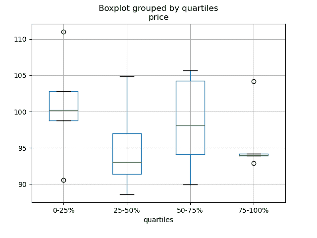
按分层变量的四分位数绘制箱线图

In [186]: df = pd.DataFrame(.....:    {.....:        "stratifying_var": np.random.uniform(0, 100, 20),.....:        "price": np.random.normal(100, 5, 20),.....:    }.....: ).....: In [187]: df["quartiles"] = pd.qcut(.....:    df["stratifying_var"], 4, labels=["0-25%", "25-50%", "50-75%", "75-100%"].....: ).....: In [188]: df.boxplot(column="price", by="quartiles")
Out[188]: <Axes: title={'center': 'price'}, xlabel='quartiles'>

../_images/quartile_boxplot.png

数据输入/输出

SQL 与 HDF5 的性能比较

CSV

CSV 文档

read_csv 的应用

追加到 csv

逐块读取 csv

逐块读取 csv 仅选择特定行

读取框架的前几行

读取一个被压缩但不是由gzip/bz2（read_csv理解的原生压缩格式）压缩的文件。这个例子展示了一个WinZipped文件，但是是在上下文管理器中打开文件并使用该句柄读取的一般应用。看这里

从文件推断数据类型

处理错误行 GH 2886

写入多行索引 CSV 而不写入重复项

读取多个文件以创建单个 DataFrame

将多个文件合并为单个 DataFrame 的最佳方法是逐个读取各个框架，将所有单个框架放入列表中，然后使用pd.concat()组合列表中的框架：

In [189]: for i in range(3):.....:    data = pd.DataFrame(np.random.randn(10, 4)).....:    data.to_csv("file_{}.csv".format(i)).....: In [190]: files = ["file_0.csv", "file_1.csv", "file_2.csv"]In [191]: result = pd.concat([pd.read_csv(f) for f in files], ignore_index=True)

您可以使用相同的方法来读取匹配模式的所有文件。这是一个使用glob的示例：

In [192]: import globIn [193]: import osIn [194]: files = glob.glob("file_*.csv")In [195]: result = pd.concat([pd.read_csv(f) for f in files], ignore_index=True)

最后，这种策略将适用于其他在 io 文档中描述的pd.read_*(...)函数。

解析多列中的日期组件

在多列中解析日期组件使用格式更快

In [196]: i = pd.date_range("20000101", periods=10000)In [197]: df = pd.DataFrame({"year": i.year, "month": i.month, "day": i.day})In [198]: df.head()
Out[198]: year  month  day
0  2000      1    1
1  2000      1    2
2  2000      1    3
3  2000      1    4
4  2000      1    5In [199]: %timeit pd.to_datetime(df.year * 10000 + df.month * 100 + df.day, format='%Y%m%d').....: ds = df.apply(lambda x: "%04d%02d%02d" % (x["year"], x["month"], x["day"]), axis=1).....: ds.head().....: %timeit pd.to_datetime(ds).....: 
4.01 ms +- 635 us per loop (mean +- std. dev. of 7 runs, 100 loops each)
1.05 ms +- 7.39 us per loop (mean +- std. dev. of 7 runs, 1,000 loops each)

在标题和数据之间跳过行

In [200]: data = """;;;;.....: ;;;;.....: ;;;;.....: ;;;;.....: ;;;;.....: ;;;;.....: ;;;;.....: ;;;;.....: ;;;;.....: ;;;;.....: date;Param1;Param2;Param4;Param5.....:    ;m²;°C;m²;m.....: ;;;;.....: 01.01.1990 00:00;1;1;2;3.....: 01.01.1990 01:00;5;3;4;5.....: 01.01.1990 02:00;9;5;6;7.....: 01.01.1990 03:00;13;7;8;9.....: 01.01.1990 04:00;17;9;10;11.....: 01.01.1990 05:00;21;11;12;13.....: """.....:

选项 1：显式传递行以跳过行

In [201]: from io import StringIOIn [202]: pd.read_csv(.....:    StringIO(data),.....:    sep=";",.....:    skiprows=[11, 12],.....:    index_col=0,.....:    parse_dates=True,.....:    header=10,.....: ).....: 
Out[202]: Param1  Param2  Param4  Param5
date 
1990-01-01 00:00:00       1       1       2       3
1990-01-01 01:00:00       5       3       4       5
1990-01-01 02:00:00       9       5       6       7
1990-01-01 03:00:00      13       7       8       9
1990-01-01 04:00:00      17       9      10      11
1990-01-01 05:00:00      21      11      12      13

选项 2：先读取列名，然后读取数据

In [203]: pd.read_csv(StringIO(data), sep=";", header=10, nrows=10).columns
Out[203]: Index(['date', 'Param1', 'Param2', 'Param4', 'Param5'], dtype='object')In [204]: columns = pd.read_csv(StringIO(data), sep=";", header=10, nrows=10).columnsIn [205]: pd.read_csv(.....:    StringIO(data), sep=";", index_col=0, header=12, parse_dates=True, names=columns.....: ).....: 
Out[205]: Param1  Param2  Param4  Param5
date 
1990-01-01 00:00:00       1       1       2       3
1990-01-01 01:00:00       5       3       4       5
1990-01-01 02:00:00       9       5       6       7
1990-01-01 03:00:00      13       7       8       9
1990-01-01 04:00:00      17       9      10      11
1990-01-01 05:00:00      21      11      12      13 
```### SQLSQL 文档[使用 SQL 从数据库中读取数据](https://stackoverflow.com/questions/10065051/python-pandas-and-databases-like-mysql)  ### ExcelExcel 文档[从类文件句柄中读取](https://stackoverflow.com/questions/15588713/sheets-of-excel-workbook-from-a-url-into-a-pandas-dataframe)[修改 XlsxWriter 输出中的格式](https://pbpython.com/improve-pandas-excel-output.html)仅加载可见工作表 [GH 19842#issuecomment-892150745](https://github.com/pandas-dev/pandas/issues/19842#issuecomment-892150745)  ### HTML[从无法处理默认请求标头的服务器中读取 HTML 表格](https://stackoverflow.com/a/18939272/564538)  ### HDFStoreHDFStores 文档[使用时间戳索引进行简单查询](https://stackoverflow.com/questions/13926089/selecting-columns-from-pandas-hdfstore-table)使用链接的多表层次结构管理异构数据 [GH 3032](https://github.com/pandas-dev/pandas/issues/3032)[合并具有数百万行的磁盘表](https://stackoverflow.com/questions/14614512/merging-two-tables-with-millions-of-rows-in-python/14617925#14617925)[在多个进程/线程从多个进程/线程写入存储时避免不一致性](https://stackoverflow.com/a/29014295/2858145)通过块来去重大型存储，本质上是一个递归减少操作。展示了一个从 csv 文件中获取数据并按块创建存储的函数，同时进行日期解析。[点击这里查看](https://stackoverflow.com/questions/16110252/need-to-compare-very-large-files-around-1-5gb-in-python/16110391#16110391)[逐块从 csv 文件创建存储](https://stackoverflow.com/questions/20428355/appending-column-to-frame-of-hdf-file-in-pandas/20428786#20428786)[在创建唯一索引的同时向存储追加数据](https://stackoverflow.com/questions/16997048/how-does-one-append-large-amounts-of-data-to-a-pandas-hdfstore-and-get-a-natural/16999397#16999397)[大数据工作流程](https://stackoverflow.com/q/14262433)[读取一系列文件，然后在追加时为存储提供全局唯一索引](https://stackoverflow.com/questions/16997048/how-does-one-append-large-amounts-of-data-to-a-pandas-hdfstore-and-get-a-natural)[在 HDFStore 上进行低组密度的 Groupby](https://stackoverflow.com/questions/15798209/pandas-group-by-query-on-large-data-in-hdfstore)[在 HDFStore 上进行高组密度的 Groupby](https://stackoverflow.com/questions/25459982/trouble-with-grouby-on-millions-of-keys-on-a-chunked-file-in-python-pandas/25471765#25471765)[在 HDFStore 上进行分层查询](https://stackoverflow.com/questions/22777284/improve-query-performance-from-a-large-hdfstore-table-with-pandas/22820780#22820780)[在 HDFStore 上进行计数](https://stackoverflow.com/questions/20497897/converting-dict-of-dicts-into-pandas-dataframe-memory-issues)[排除 HDFStore 异常](https://stackoverflow.com/questions/15488809/how-to-trouble-shoot-hdfstore-exception-cannot-find-the-correct-atom-type)[使用字符串设置 min_itemsize](https://stackoverflow.com/questions/15988871/hdfstore-appendstring-dataframe-fails-when-string-column-contents-are-longer)[使用 ptrepack 在存储上创建完全排序的索引](https://stackoverflow.com/questions/17893370/ptrepack-sortby-needs-full-index)将属性存储到组节点```py
In [206]: df = pd.DataFrame(np.random.randn(8, 3))In [207]: store = pd.HDFStore("test.h5")In [208]: store.put("df", df)# you can store an arbitrary Python object via pickle
In [209]: store.get_storer("df").attrs.my_attribute = {"A": 10}In [210]: store.get_storer("df").attrs.my_attribute
Out[210]: {'A': 10}

你可以通过将 driver 参数传递给 PyTables 来在内存中创建或加载 HDFStore。只有在关闭 HDFStore 时才会将更改写入磁盘。

In [211]: store = pd.HDFStore("test.h5", "w", driver="H5FD_CORE")In [212]: df = pd.DataFrame(np.random.randn(8, 3))In [213]: store["test"] = df# only after closing the store, data is written to disk:
In [214]: store.close() 
```### 二进制文件pandas 可以轻松接受 NumPy 记录数组，如果你需要读取由 C 结构数组组成的二进制文件。例如，给定一个名为 `main.c` 的 C 程序，在 64 位机器上使用 `gcc main.c -std=gnu99` 编译，```py
#include  <stdio.h>
#include  <stdint.h>typedef  struct  _Data
{int32_t  count;double  avg;float  scale;
}  Data;int  main(int  argc,  const  char  *argv[])
{size_t  n  =  10;Data  d[n];for  (int  i  =  0;  i  <  n;  ++i){d[i].count  =  i;d[i].avg  =  i  +  1.0;d[i].scale  =  (float)  i  +  2.0f;}FILE  *file  =  fopen("binary.dat",  "wb");fwrite(&d,  sizeof(Data),  n,  file);fclose(file);return  0;
}

以下 Python 代码将把二进制文件 'binary.dat' 读入 pandas 的 DataFrame，其中结构的每个元素对应于框架中的一列：

names = "count", "avg", "scale"# note that the offsets are larger than the size of the type because of
# struct padding
offsets = 0, 8, 16
formats = "i4", "f8", "f4"
dt = np.dtype({"names": names, "offsets": offsets, "formats": formats}, align=True)
df = pd.DataFrame(np.fromfile("binary.dat", dt))

注意

结构元素的偏移量可能会因文件创建时所用机器的架构而异。不建议使用这种原始二进制文件格式进行通用数据存储，因为它不跨平台。我们建议使用 HDF5 或 parquet，这两种格式都受到 pandas 的 IO 功能支持。### CSV

CSV 文档

read_csv 演示

追加到 csv

逐块读取 csv

逐块读取 csv 中的特定行

读取框架的前几行

读取已压缩但不是由 gzip/bz2（read_csv 理解的原生压缩格式）压缩的文件。此示例展示了一个 WinZipped 文件，但是是在上下文管理器中打开文件并使用该句柄进行读取的一般应用。点击这里查看

从文件推断数据类型

处理错误行 GH 2886

写入具有多行索引的 CSV，避免写入重复行

读取多个文件以创建单个 DataFrame

将多个文件合并为单个 DataFrame 的最佳方法是逐个读取各个框架，将所有单独的框架放入列表中，然后使用 pd.concat() 组合列表中的框架：

In [189]: for i in range(3):.....:    data = pd.DataFrame(np.random.randn(10, 4)).....:    data.to_csv("file_{}.csv".format(i)).....: In [190]: files = ["file_0.csv", "file_1.csv", "file_2.csv"]In [191]: result = pd.concat([pd.read_csv(f) for f in files], ignore_index=True)

您可以使用相同的方法来读取所有匹配模式的文件。以下是使用 glob 的示例：

In [192]: import globIn [193]: import osIn [194]: files = glob.glob("file_*.csv")In [195]: result = pd.concat([pd.read_csv(f) for f in files], ignore_index=True)

最后，这种策略将适用于 io 文档中描述的其他 pd.read_*(...) 函数。

解析多列中的日期组件

使用格式解析多列中的日期组件更快

In [196]: i = pd.date_range("20000101", periods=10000)In [197]: df = pd.DataFrame({"year": i.year, "month": i.month, "day": i.day})In [198]: df.head()
Out[198]: year  month  day
0  2000      1    1
1  2000      1    2
2  2000      1    3
3  2000      1    4
4  2000      1    5In [199]: %timeit pd.to_datetime(df.year * 10000 + df.month * 100 + df.day, format='%Y%m%d').....: ds = df.apply(lambda x: "%04d%02d%02d" % (x["year"], x["month"], x["day"]), axis=1).....: ds.head().....: %timeit pd.to_datetime(ds).....: 
4.01 ms +- 635 us per loop (mean +- std. dev. of 7 runs, 100 loops each)
1.05 ms +- 7.39 us per loop (mean +- std. dev. of 7 runs, 1,000 loops each)

在标题和数据之间跳过行

In [200]: data = """;;;;.....: ;;;;.....: ;;;;.....: ;;;;.....: ;;;;.....: ;;;;.....: ;;;;.....: ;;;;.....: ;;;;.....: ;;;;.....: date;Param1;Param2;Param4;Param5.....:    ;m²;°C;m²;m.....: ;;;;.....: 01.01.1990 00:00;1;1;2;3.....: 01.01.1990 01:00;5;3;4;5.....: 01.01.1990 02:00;9;5;6;7.....: 01.01.1990 03:00;13;7;8;9.....: 01.01.1990 04:00;17;9;10;11.....: 01.01.1990 05:00;21;11;12;13.....: """.....:

选项 1：显式传递要跳过的行数

In [201]: from io import StringIOIn [202]: pd.read_csv(.....:    StringIO(data),.....:    sep=";",.....:    skiprows=[11, 12],.....:    index_col=0,.....:    parse_dates=True,.....:    header=10,.....: ).....: 
Out[202]: Param1  Param2  Param4  Param5
date 
1990-01-01 00:00:00       1       1       2       3
1990-01-01 01:00:00       5       3       4       5
1990-01-01 02:00:00       9       5       6       7
1990-01-01 03:00:00      13       7       8       9
1990-01-01 04:00:00      17       9      10      11
1990-01-01 05:00:00      21      11      12      13

选项 2：先读取列名，然后读取数据

In [203]: pd.read_csv(StringIO(data), sep=";", header=10, nrows=10).columns
Out[203]: Index(['date', 'Param1', 'Param2', 'Param4', 'Param5'], dtype='object')In [204]: columns = pd.read_csv(StringIO(data), sep=";", header=10, nrows=10).columnsIn [205]: pd.read_csv(.....:    StringIO(data), sep=";", index_col=0, header=12, parse_dates=True, names=columns.....: ).....: 
Out[205]: Param1  Param2  Param4  Param5
date 
1990-01-01 00:00:00       1       1       2       3
1990-01-01 01:00:00       5       3       4       5
1990-01-01 02:00:00       9       5       6       7
1990-01-01 03:00:00      13       7       8       9
1990-01-01 04:00:00      17       9      10      11
1990-01-01 05:00:00      21      11      12      13

读取多个文件以创建单个 DataFrame

将多个文件合并为单个 DataFrame 的最佳方法是逐个读取各个框架，将所有单独的框架放入列表中，然后使用 pd.concat() 组合列表中的框架：

In [189]: for i in range(3):.....:    data = pd.DataFrame(np.random.randn(10, 4)).....:    data.to_csv("file_{}.csv".format(i)).....: In [190]: files = ["file_0.csv", "file_1.csv", "file_2.csv"]In [191]: result = pd.concat([pd.read_csv(f) for f in files], ignore_index=True)

您可以使用相同的方法来读取所有匹配模式的文件。以下是使用 glob 的示例：

In [192]: import globIn [193]: import osIn [194]: files = glob.glob("file_*.csv")In [195]: result = pd.concat([pd.read_csv(f) for f in files], ignore_index=True)

最后，这种策略将适用于 io 文档中描述的其他 pd.read_*(...) 函数。

解析多列中的日期组件

在多列中解析日期组件时，使用格式更快

In [196]: i = pd.date_range("20000101", periods=10000)In [197]: df = pd.DataFrame({"year": i.year, "month": i.month, "day": i.day})In [198]: df.head()
Out[198]: year  month  day
0  2000      1    1
1  2000      1    2
2  2000      1    3
3  2000      1    4
4  2000      1    5In [199]: %timeit pd.to_datetime(df.year * 10000 + df.month * 100 + df.day, format='%Y%m%d').....: ds = df.apply(lambda x: "%04d%02d%02d" % (x["year"], x["month"], x["day"]), axis=1).....: ds.head().....: %timeit pd.to_datetime(ds).....: 
4.01 ms +- 635 us per loop (mean +- std. dev. of 7 runs, 100 loops each)
1.05 ms +- 7.39 us per loop (mean +- std. dev. of 7 runs, 1,000 loops each)

在标题和数据之间跳过行

In [200]: data = """;;;;.....: ;;;;.....: ;;;;.....: ;;;;.....: ;;;;.....: ;;;;.....: ;;;;.....: ;;;;.....: ;;;;.....: ;;;;.....: date;Param1;Param2;Param4;Param5.....:    ;m²;°C;m²;m.....: ;;;;.....: 01.01.1990 00:00;1;1;2;3.....: 01.01.1990 01:00;5;3;4;5.....: 01.01.1990 02:00;9;5;6;7.....: 01.01.1990 03:00;13;7;8;9.....: 01.01.1990 04:00;17;9;10;11.....: 01.01.1990 05:00;21;11;12;13.....: """.....:

选项 1：显式传递行以跳过行

In [201]: from io import StringIOIn [202]: pd.read_csv(.....:    StringIO(data),.....:    sep=";",.....:    skiprows=[11, 12],.....:    index_col=0,.....:    parse_dates=True,.....:    header=10,.....: ).....: 
Out[202]: Param1  Param2  Param4  Param5
date 
1990-01-01 00:00:00       1       1       2       3
1990-01-01 01:00:00       5       3       4       5
1990-01-01 02:00:00       9       5       6       7
1990-01-01 03:00:00      13       7       8       9
1990-01-01 04:00:00      17       9      10      11
1990-01-01 05:00:00      21      11      12      13

选项 2：先读取列名，然后读取数据

In [203]: pd.read_csv(StringIO(data), sep=";", header=10, nrows=10).columns
Out[203]: Index(['date', 'Param1', 'Param2', 'Param4', 'Param5'], dtype='object')In [204]: columns = pd.read_csv(StringIO(data), sep=";", header=10, nrows=10).columnsIn [205]: pd.read_csv(.....:    StringIO(data), sep=";", index_col=0, header=12, parse_dates=True, names=columns.....: ).....: 
Out[205]: Param1  Param2  Param4  Param5
date 
1990-01-01 00:00:00       1       1       2       3
1990-01-01 01:00:00       5       3       4       5
1990-01-01 02:00:00       9       5       6       7
1990-01-01 03:00:00      13       7       8       9
1990-01-01 04:00:00      17       9      10      11
1990-01-01 05:00:00      21      11      12      13

选项 1：显式传递行以跳过行

In [201]: from io import StringIOIn [202]: pd.read_csv(.....:    StringIO(data),.....:    sep=";",.....:    skiprows=[11, 12],.....:    index_col=0,.....:    parse_dates=True,.....:    header=10,.....: ).....: 
Out[202]: Param1  Param2  Param4  Param5
date 
1990-01-01 00:00:00       1       1       2       3
1990-01-01 01:00:00       5       3       4       5
1990-01-01 02:00:00       9       5       6       7
1990-01-01 03:00:00      13       7       8       9
1990-01-01 04:00:00      17       9      10      11
1990-01-01 05:00:00      21      11      12      13

选项 2：先读取列名，然后读取数据

In [203]: pd.read_csv(StringIO(data), sep=";", header=10, nrows=10).columns
Out[203]: Index(['date', 'Param1', 'Param2', 'Param4', 'Param5'], dtype='object')In [204]: columns = pd.read_csv(StringIO(data), sep=";", header=10, nrows=10).columnsIn [205]: pd.read_csv(.....:    StringIO(data), sep=";", index_col=0, header=12, parse_dates=True, names=columns.....: ).....: 
Out[205]: Param1  Param2  Param4  Param5
date 
1990-01-01 00:00:00       1       1       2       3
1990-01-01 01:00:00       5       3       4       5
1990-01-01 02:00:00       9       5       6       7
1990-01-01 03:00:00      13       7       8       9
1990-01-01 04:00:00      17       9      10      11
1990-01-01 05:00:00      21      11      12      13

SQL

SQL 文档

使用 SQL 从数据库中读取数据

Excel

Excel 文档

从类文件句柄读取

修改 XlsxWriter 输出中的格式

仅加载可见工作表 GH 19842#issuecomment-892150745

HTML

从无法处理默认请求头的服务器读取 HTML 表格

HDFStore

HDFStores 文档

使用时间戳索引进行简单查询

使用链接的多表层次结构管理异构数据 GH 3032

合并具有数百万行的磁盘上的表

在多个进程/线程从多个进程/线程写入存储时避免不一致性

通过块对大型存储进行去重，本质上是一个递归减少操作。展示了一个从 csv 文件中接收数据并按块创建存储的函数，同时也进行了日期解析。点击这里查看

从 csv 文件逐块创建存储

在创建唯一索引的同时向存储追加数据

大数据工作流

读取一系列文件，然后在追加时为存储提供全局唯一索引

在具有低组密度的 HDFStore 上进行分组

在具有高组密度的 HDFStore 上进行分组

在 HDFStore 上进行分层查询

使用 HDFStore 进行计数

解决 HDFStore 异常

使用字符串设置 min_itemsize

使用 ptrepack 在存储上创建完全排序的索引

将属性存储到组节点

In [206]: df = pd.DataFrame(np.random.randn(8, 3))In [207]: store = pd.HDFStore("test.h5")In [208]: store.put("df", df)# you can store an arbitrary Python object via pickle
In [209]: store.get_storer("df").attrs.my_attribute = {"A": 10}In [210]: store.get_storer("df").attrs.my_attribute
Out[210]: {'A': 10}

通过将 driver 参数传递给 PyTables，可以在内存中创建或加载 HDFStore。只有在关闭 HDFStore 时才会将更改写入磁盘。

In [211]: store = pd.HDFStore("test.h5", "w", driver="H5FD_CORE")In [212]: df = pd.DataFrame(np.random.randn(8, 3))In [213]: store["test"] = df# only after closing the store, data is written to disk:
In [214]: store.close()

二进制文件

如果需要读取由 C 结构数组组成的二进制文件，pandas 可以轻松接受 NumPy 记录数组。例如，给定一个名为 main.c 的文件中的 C 程序，在 64 位机器上使用 gcc main.c -std=gnu99 编译，

#include  <stdio.h>
#include  <stdint.h>typedef  struct  _Data
{int32_t  count;double  avg;float  scale;
}  Data;int  main(int  argc,  const  char  *argv[])
{size_t  n  =  10;Data  d[n];for  (int  i  =  0;  i  <  n;  ++i){d[i].count  =  i;d[i].avg  =  i  +  1.0;d[i].scale  =  (float)  i  +  2.0f;}FILE  *file  =  fopen("binary.dat",  "wb");fwrite(&d,  sizeof(Data),  n,  file);fclose(file);return  0;
}

以下 Python 代码将二进制文件 'binary.dat' 读入 pandas 的 DataFrame 中，结构的每个元素对应帧中的一列：

names = "count", "avg", "scale"# note that the offsets are larger than the size of the type because of
# struct padding
offsets = 0, 8, 16
formats = "i4", "f8", "f4"
dt = np.dtype({"names": names, "offsets": offsets, "formats": formats}, align=True)
df = pd.DataFrame(np.fromfile("binary.dat", dt))

注意

结构元素的偏移量可能因创建文件的机器架构而异。不建议使用这种原始二进制文件格式进行通用数据存储，因为它不跨平台。我们建议使用 HDF5 或 parquet，这两者都受到 pandas IO 设施的支持。

计算

时间序列的数值积分（基于样本）

时间增量

时间增量文档。

使用时间差

In [222]: import datetimeIn [223]: s = pd.Series(pd.date_range("2012-1-1", periods=3, freq="D"))In [224]: s - s.max()
Out[224]: 
0   -2 days
1   -1 days
2    0 days
dtype: timedelta64[ns]In [225]: s.max() - s
Out[225]: 
0   2 days
1   1 days
2   0 days
dtype: timedelta64[ns]In [226]: s - datetime.datetime(2011, 1, 1, 3, 5)
Out[226]: 
0   364 days 20:55:00
1   365 days 20:55:00
2   366 days 20:55:00
dtype: timedelta64[ns]In [227]: s + datetime.timedelta(minutes=5)
Out[227]: 
0   2012-01-01 00:05:00
1   2012-01-02 00:05:00
2   2012-01-03 00:05:00
dtype: datetime64[ns]In [228]: datetime.datetime(2011, 1, 1, 3, 5) - s
Out[228]: 
0   -365 days +03:05:00
1   -366 days +03:05:00
2   -367 days +03:05:00
dtype: timedelta64[ns]In [229]: datetime.timedelta(minutes=5) + s
Out[229]: 
0   2012-01-01 00:05:00
1   2012-01-02 00:05:00
2   2012-01-03 00:05:00
dtype: datetime64[ns]

添加和减去时间差和日期

In [230]: deltas = pd.Series([datetime.timedelta(days=i) for i in range(3)])In [231]: df = pd.DataFrame({"A": s, "B": deltas})In [232]: df
Out[232]: A      B
0 2012-01-01 0 days
1 2012-01-02 1 days
2 2012-01-03 2 daysIn [233]: df["New Dates"] = df["A"] + df["B"]In [234]: df["Delta"] = df["A"] - df["New Dates"]In [235]: df
Out[235]: A      B  New Dates   Delta
0 2012-01-01 0 days 2012-01-01  0 days
1 2012-01-02 1 days 2012-01-03 -1 days
2 2012-01-03 2 days 2012-01-05 -2 daysIn [236]: df.dtypes
Out[236]: 
A             datetime64[ns]
B            timedelta64[ns]
New Dates     datetime64[ns]
Delta        timedelta64[ns]
dtype: object

另一个示例

可以使用 np.nan 将值设置为 NaT，类似于 datetime

In [237]: y = s - s.shift()In [238]: y
Out[238]: 
0      NaT
1   1 days
2   1 days
dtype: timedelta64[ns]In [239]: y[1] = np.nanIn [240]: y
Out[240]: 
0      NaT
1      NaT
2   1 days
dtype: timedelta64[ns]

创建示例数据

要从给定值的每个组合创建数据框，类似于 R 的expand.grid()函数，我们可以创建一个字典，其中键是列名，值是数据值的列表：

In [241]: def expand_grid(data_dict):.....:    rows = itertools.product(*data_dict.values()).....:    return pd.DataFrame.from_records(rows, columns=data_dict.keys()).....: In [242]: df = expand_grid(.....:    {"height": [60, 70], "weight": [100, 140, 180], "sex": ["Male", "Female"]}.....: ).....: In [243]: df
Out[243]: height  weight     sex
0       60     100    Male
1       60     100  Female
2       60     140    Male
3       60     140  Female
4       60     180    Male
5       60     180  Female
6       70     100    Male
7       70     100  Female
8       70     140    Male
9       70     140  Female
10      70     180    Male
11      70     180  Female

恒定系列

要评估一个系列是否具有恒定值，我们可以检查series.nunique() <= 1。然而，一种更高效的方法，不需要首先计算所有唯一值，是：

In [244]: v = s.to_numpy()In [245]: is_constant = v.shape[0] == 0 or (s[0] == s).all()

此方法假定系列不包含缺失值。对于我们将删除 NA 值的情况，我们可以先简单地删除这些值：

In [246]: v = s.dropna().to_numpy()In [247]: is_constant = v.shape[0] == 0 or (s[0] == s).all()

如果缺失值被视为与任何其他值不同，则可以使用：

In [248]: v = s.to_numpy()In [249]: is_constant = v.shape[0] == 0 or (s[0] == s).all() or not pd.notna(v).any()

（请注意，此示例不区分np.nan、pd.NA和None之间的差异）