1 统计指标

• 随机变量$X$的理论平均值称为期望: $\mu =E(X)$
• 但现实中通常不知道$\mu$, 因此使用已知样本来获取均值
  $$\overline{X}=\frac{1}{n}\sum _{i=1}^n{X}_i.$$
• 方差variance定义为：
  $${\sigma }^2=E(|X-\mu {|}^2).$$
• 用已知样本的数据来代替:
  $$S^2=Var(X)=\frac{1}{n}\sum _{i=1}^n(X_i-\mu {)}^2.$$
• 由于$\mu$未知, 使用贝塞尔校正：
  $$S^2=Var(X)=\frac{1}{n-1}\sum _{i=1}^n(X_i-\overline{X}{)}^2.$$
• 原因: 在已知数据上, 使用$\overline{X}$获得的结果一般更小：
  $$\sum _{i=1}^{n-1}(X_i-\overline{X}{)}^2\le \sum _{i=1}^{n-1}(X_i-\mu {)}^2.$$
• 更多解释: https://www.zhihu.com/question/20099757
• 标准差：
  $${\sigma }_X=S=\sqrt{Var(X)}.$$

偏差与方差：

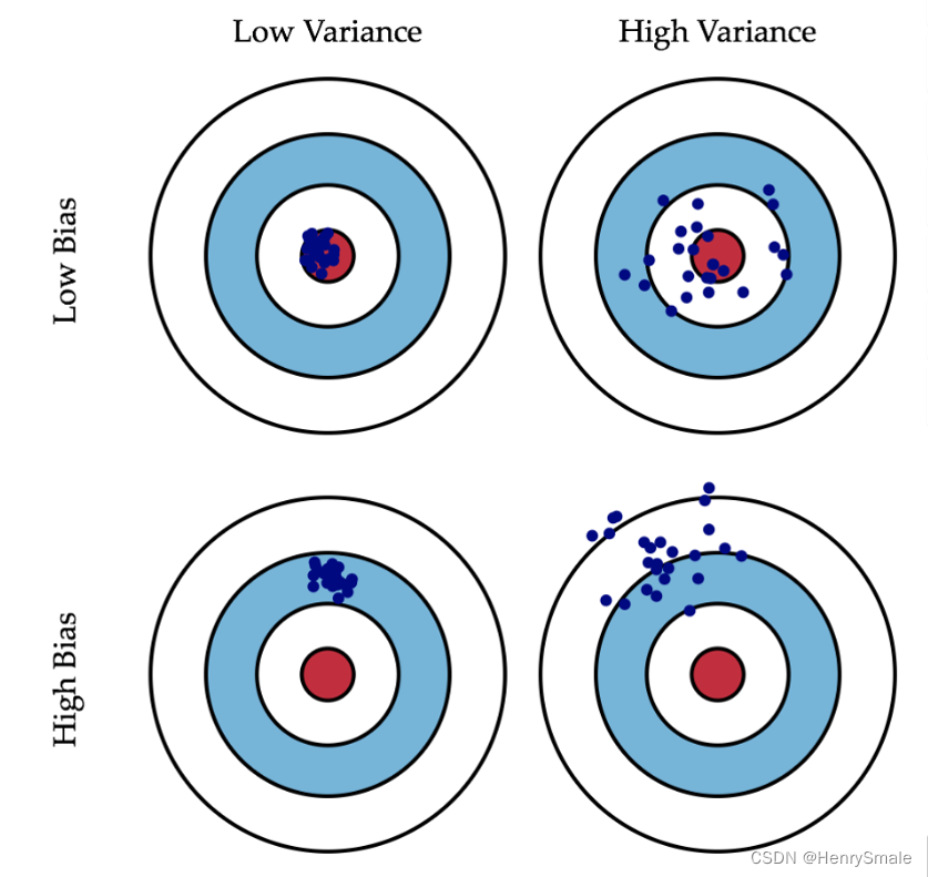
• 方差(again)
  $$Var(X)={\sigma }_X^2=\frac{1}{n-1}\sum _{i=1}^n(X_i-\overline{X})(X_i-\overline{X}).$$
• 协方差
  $$Cov(X,Y)=\frac{1}{n-1}\sum _{i=1}^n(X_i-\overline{X})(Y_i-\overline{Y}).$$
• Pearson相关系数
  $$Corr(X,Y)={\rho }_{X,Y}=\frac{Cov(X,Y)}{{\sigma }_X{\sigma }_Y}.$$

2 线性回归

2.1 回归任务

分类与回归

• 分类任务预测类别，即是/否等离散值：如是否生病;
• 回归任务预测实型值：如气温

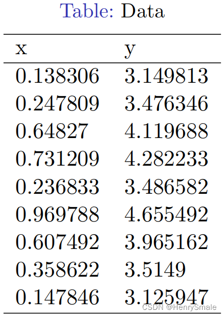
拟合空间中的点 (注意数据点没有类别标记, 输出也占一维):

• 一个条件属性：直线;
• 两个条件属性：平面;
• 更多条件属性：超平面.

拟合线:

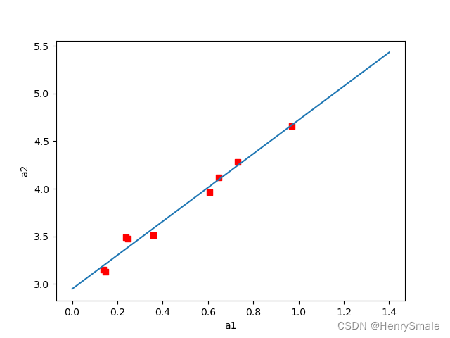
2.2 最小二乘法

线性分割面的表达

• 平面几何表达直线(两个系数):
  $$y=ax+b.$$
• 重新命名变量:
  $$w_0+w_1{x}_1=y.$$
• 强行加一个$x_0\equiv 1$:
  $$w_0{x}_0+w_1{x}_1=y.$$
• 向量表达：
  $$\mathbf{xw}=y$$

与Logistic regression相比: $\mathbf{w}$和$\mathbf{x}$均少了一维。

损失函数
$$\sum _{i=1}^m({\mathbf{x}}_i\mathbf{w}-y_i{)}^2.$$
矩阵化的表达：
$$\Vert \mathbf{Xw}-\mathbf{Y}{\Vert }^2.$$
矩阵化的展开式：
$$L(\mathbf{X},\mathbf{Y},\mathbf{w})=(\mathbf{Xw}-\mathbf{Y}{)}^{\mathrm{T}}(\mathbf{Xw}-\mathbf{Y}).$$
求解推导
$$\begin{array}{l}L(\mathbf{X},\mathbf{Y},\mathbf{w})\\ =(\mathbf{Xw}-\mathbf{Y}{)}^{\mathrm{T}}(\mathbf{Xw}-\mathbf{Y})\\ =({\mathbf{w}}^{\mathrm{T}}{\mathbf{X}}^{\mathrm{T}}-{\mathbf{Y}}^{\mathrm{T}})(\mathbf{Xw}-\mathbf{Y})\\ ={\mathbf{w}}^{\mathrm{T}}{\mathbf{X}}^{\mathrm{T}}\mathbf{Xw}-{\mathbf{w}}^{\mathrm{T}}{\mathbf{X}}^{\mathrm{T}}\mathbf{Y}-{\mathbf{Y}}^{\mathrm{T}}\mathbf{Xw}+{\mathbf{Y}}^{\mathrm{T}}\mathbf{Y}\end{array}$$
为最小化该函数, 应对$\mathbf{w}$求导, 且其结果为0。
根据矩阵求导法则：
$$\begin{array}{l}\frac{\partial A\mathbf{w}}{\partial \mathbf{w}}=A,\\ \frac{\partial {\mathbf{w}}^{\mathrm{T}}A}{\partial \mathbf{w}}=A^{\mathrm{T}},\\ \frac{\partial {\mathbf{w}}^{\mathrm{T}}A\mathbf{w}}{\partial \mathbf{w}}=2{\mathbf{w}}^{\mathrm{T}}A.\end{array}$$
可知：
$$\begin{array}{l}\frac{\partial L(\mathbf{X},\mathbf{Y},\mathbf{w})}{\partial \mathbf{w}}\\ =\frac{\partial {\mathbf{w}}^{\mathrm{T}}{\mathbf{X}}^{\mathrm{T}}\mathbf{Xw}}{\partial \mathbf{w}}-\frac{\partial {\mathbf{w}}^{\mathrm{T}}{\mathbf{X}}^{\mathrm{T}}\mathbf{Y}}{\partial \mathbf{w}}-\frac{\partial {\mathbf{Y}}^{\mathrm{T}}\mathbf{Xw}}{\partial \mathbf{w}}+\frac{\partial {\mathbf{Y}}^{\mathrm{T}}\mathbf{Y}}{\partial \mathbf{w}}\\ =2{\mathbf{w}}^{\mathrm{T}}{\mathbf{X}}^{\mathrm{T}}\mathbf{X}-{\mathbf{Y}}^{\mathrm{T}}\mathbf{X}-{\mathbf{Y}}^{\mathrm{T}}\mathbf{X}+0\\ =2{\mathbf{w}}^{\mathrm{T}}{\mathbf{X}}^{\mathrm{T}}\mathbf{X}-2{\mathbf{Y}}^{\mathrm{T}}\mathbf{X}\end{array}$$
由
$$2{\hat{\mathbf{w}}}^{\mathrm{T}}{\mathbf{X}}^{\mathrm{T}}\mathbf{X}-2{\mathbf{Y}}^{\mathrm{T}}\mathbf{X}=0,$$
可得
$${\hat{\mathbf{w}}}^{\mathrm{T}}{\mathbf{X}}^{\mathrm{T}}\mathbf{X}={\mathbf{Y}}^{\mathrm{T}}\mathbf{X}.$$
两边转置
$${\mathbf{X}}^{\mathrm{T}}\mathbf{X}\hat{\mathbf{w}}={\mathbf{X}}^{\mathrm{T}}\mathbf{Y}.$$
最后
$$\hat{\mathbf{w}}=({\mathbf{X}}^{\mathrm{T}}\mathbf{X}{)}^{-1}{\mathbf{X}}^{\mathrm{T}}\mathbf{Y}.$$

2.3 代码分析

#Test my implemenation of Logistic regression and existing one.
import time
#import sklearn, sklearn.datasets, sklearn.neighbors, sklearn.linear_model
import matplotlib.pyplot as plt
import numpy as np"""
Train a regressor
"""
def linearRegression(X, Y):weights = (X.T * X).I * X.T * Yreturn weights"""
函数：画出决策边界，仅为演示用，且仅支持两个条件属性的数据
"""
def plotBestFit(paraWeights):X, Y = loadDataset()dataArr = np.array(X)x1 = [x[1] for x in dataArr]print("x1 = ", x1)y1 = np.array(Y)fig=plt.figure()ax=fig.add_subplot(111)ax.scatter(x1, y1,s=30,c='red',marker='s')#画出拟合直线x = np.arange(0, 1.5, 0.1)y = paraWeights[0] + paraWeights[1]*x    #直线满足关系：y = w0 + w1 xax.plot(x,y)plt.xlabel('a1')plt.ylabel('a2')plt.show()"""
读数据, csv格式
"""
def loadDataset(paraFilename="data/regression-example01.csv"):dataMat=[]  #列表listlabelMat=[]txt=open(paraFilename)for line in txt.readlines():tempValuesStringArray = np.array(line.replace("\n", "").split(','))tempValues = [float(tempValue) for tempValue in tempValuesStringArray]tempArray = [1.0] + [tempValue for tempValue in tempValues]tempx = tempArray[:-1] #不要最后一列tempy = tempArray[-1] #仅最后一列dataMat.append(tempx)labelMat.append(tempy)print("dataMat = ", dataMat)print("labelMat = ", labelMat)return np.mat(dataMat), np.mat(labelMat).T"""
Linear regression
"""
def mfLinearRegressionTest():#Step 1. Load the dataset and initialize#如果括号内不写数据，则使用4个属性前2个类别的irisX, Y = loadDataset("data/regression-example01.csv")tempStartTime = time.time()tempScore = 0numInstances = len(Y)#Step 2. Trainweights = linearRegression(X, Y)print("Weights = ", weights)tempEndTime = time.time()tempRuntime = tempEndTime - tempStartTime#Step 4. Output#print('Mf logistic socre: {}, runtime = {}'.format(tempScore, tempRuntime))#Step 5. Illustrate 仅对两个属性情况有效rowWeights = np.transpose(weights).A[0]plotBestFit(rowWeights)"""
Local linear regression for one data point
"""
def localLinearRegression(paraTestPoint, X, Y, k = 1.0):m = len(X)weights = np.mat(np.eye((m)))for j in range(m):diffMat = paraTestPoint - X[j, :]#print("diffMat = {}, diffMat^2 = {}".format(diffMat, diffMat * diffMat.T))weights[j, j] = np.exp(- diffMat * diffMat.T/(2.0 * k**2))#print("weights[{}, {}] = {}".format(j, j, weights[j, j]))#print("weights = ", weights)tempWeights = (X.T * weights * X).I * X.T  * weights * Yprediction = paraTestPoint * tempWeightsreturn prediction[0, 0]"""
局部加权回归
"""
def mfLocalLinearRegressionTest():#Step 1. Load the dataset and initialize#如果括号内不写数据，则使用4个属性前2个类别的irisX, Y = loadDataset("data/regression-example01.csv")tempStartTime = time.time()tempScore = 0numInstances = len(Y)#Step 2. Predict one by onepredicts = [0] * numInstancesfor i in range(numInstances):predicts[i] = localLinearRegression(X[i], X, Y, 0.05)#print("predicts = ", predicts)#print("Real = ", Y)tempEndTime = time.time()tempRuntime = tempEndTime - tempStartTime#Step 4. OutputplotLocalLinear(X, Y, X, predicts)"""
函数：画出决策边界，仅为演示用，且仅支持两个条件属性的数据
"""
def plotLocalLinear(paraX1, paraY1, paraX2, paraY2):#print("The data is: ", paraX1)m = len(paraY1)x1 = [paraX1[i, 1] for i in range(m)]#print("x1 = ", x1)y1 = np.array(paraY1)fig=plt.figure()ax = fig.add_subplot(111)ax.scatter(x1, y1, s = 30, c = 'red', marker = 's')#画出拟合线x2 = [paraX2[i, 1] for i in range(m)]y2 = np.array(paraY2)ax.plot(x2, y2)plt.xlabel('a1')plt.ylabel('a2')plt.show()"""
Train a ridge regressor
"""
def ridgeRegression(X, Y, paraLambda):m = len(X[0])ridge = np.mat(np.eye((m))) * 0.1weights = (X.T * X + ridge).I * X.T * Yreturn weights"""
Linear regression
"""
def mfRidgeRegressionTest():#Step 1. Load the dataset and initialize#如果括号内不写数据，则使用4个属性前2个类别的irisX, Y = loadDataset("data/regression-example01.csv")tempStartTime = time.time()tempScore = 0numInstances = len(Y)#Step 2. Trainweights = ridgeRegression(X, Y, 0.1)print("Weights = ", weights)tempEndTime = time.time()tempRuntime = tempEndTime - tempStartTime#Step 4. Output#print('Mf logistic socre: {}, runtime = {}'.format(tempScore, tempRuntime))#Step 5. Illustrate 仅对两个属性情况有效rowWeights = np.transpose(weights).A[0]plotBestFit(rowWeights)def main():mfLinearRegressionTest()#mfLocalLinearRegressionTest()mfRidgeRegressionTest()main()

3 局部线性回归

4 岭回归

5 Lasso回归

6 小结