• 问题要求

在UCI数据集上的Iris和Sonar数据上验证算法的有效性。训练和测试样本有三种方式（三选一）进行划分：

（一） 将数据随机分训练和测试，多次平均求结果

（二）K折交叉验证

（三）留1法

针对不同维数，画出曲线图。

• 问题分析

（一）数据集

1.Iris数据集是常用的分类实验数据集，由Fisher收集整理。Iris也称鸢尾花卉数据集，是一类多重变量分析的数据集。数据集包含150个数据样本，分为3类，每类50个数据，每个数据包含4个属性。可通过花萼长度，花萼宽度，花瓣长度，花瓣宽度4个属性预测鸢尾花卉属于（Setosa，Versicolour，Virginica）三个种类中的哪一类。

2.在Sonar数据集中有两类（字母“R”（岩石）和“M”（矿井）），分别有97个和111个数据，每个数据有60维的特征。这个分类任务是为了判断声纳的回传信号是来自金属圆柱还是不规则的圆柱形石头。

（二）Fisher线性判别分析

1.方法总括

Fisher线性判别方法可概括为把 d 维空间的样本投影到一条直线上，形成一维空间，即通过降维去解决两分类问题。如何根据实际数据找到一条最好的、最易于分类的投影方向，是 Fisher 判别方法所要解决的基本问题。

2. 求解过程

（1）核心思想

假设有一集合 D 包含 m 个 n 维样本{x1, x2, …, xm}，第一类样本集合记为 D1，规模为 N1，第二类样本集合记为 D2，规模为 N2。若对 xi 的分量做线性组合可得标量：yi = wTxi（i=1,2,…,m）这样便得到 m 个一维样本 yi 组成的集合， 并可分为两个子集 D’1 和 D’2。计算阈值 yo，当 yi>yo 时判断 xi 属于第一类， 当 yi<yo 时判断 xi 属于第二类，当 yi=yo 时 xi 可判给任何一类或者拒收。（2）具体推导

相关书籍或网站上都有具体推导过程，这里不再赘述。

  (3)样本划分

采用留1法划分训练集和数据集，该方法是K折法的一种极端情况。

在K折法中，将全部训练集 S分成 k个不相交的子集，假设 S中的训练样例个数为 N，那么每一个子集有 N/k 个训练样例，相应的子集称作 {s1,s2,…,sk}。每次从分好的子集中里面，拿出一个作为测试集，其它k-1个作为训练集，根据训练训练出模型或者假设函数。然后把这个模型放到测试集上，得到分类率，计算k次求得的分类率的平均值，作为该模型或者假设函数的真实分类率。

当取K的值为样本个数N时，即将每一个样本作为测试样本，其它N-1个样本作为训练样本。这样得到N个分类器，N个测试结果。用这N个结果的平均值来衡量模型的性能，这就是留1法。在UCI数据集中，由于数据个数较少，采用留一法可以使样本利用率最高。

• 仿真结果
• 1.Iris数据集

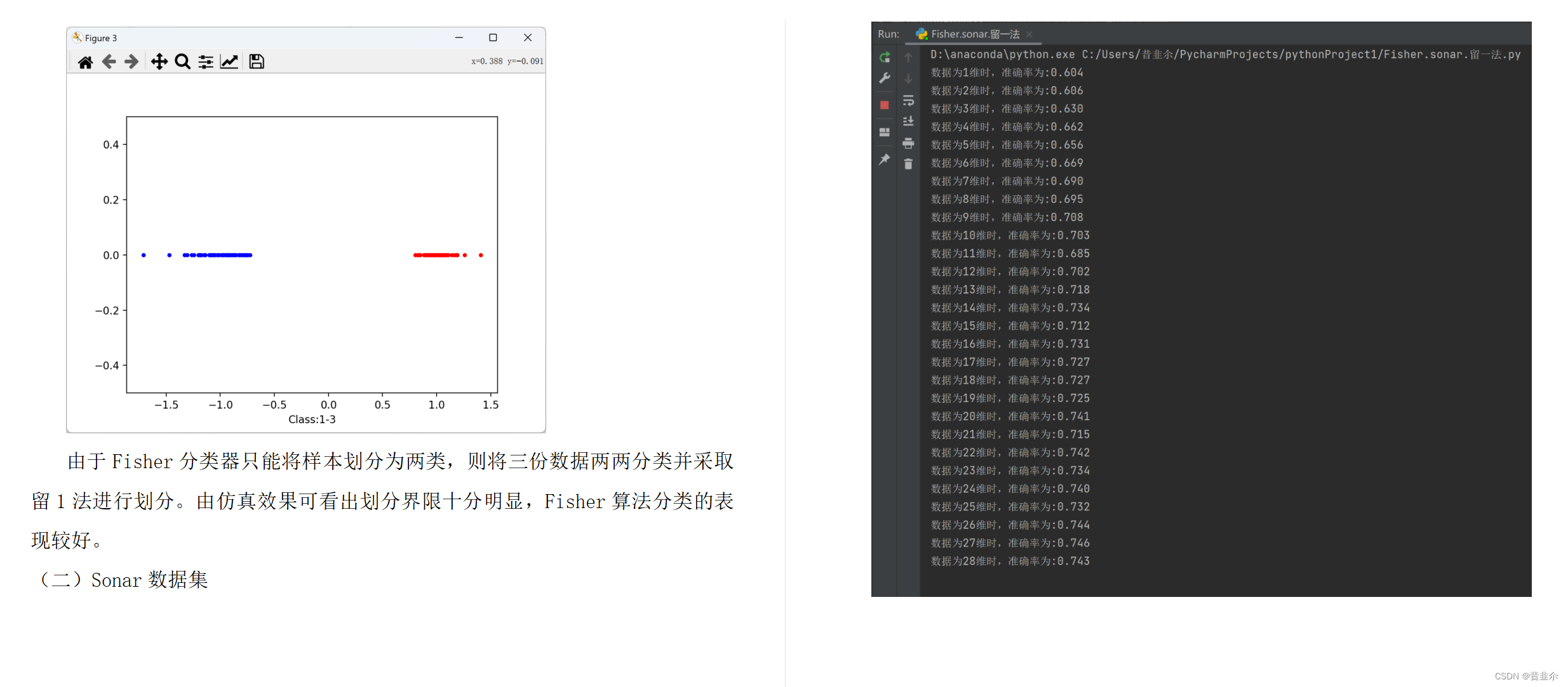
由于Fisher分类器只能将样本划分为两类，则将三份数据两两分类并采取留1法进行划分。由仿真效果可看出划分界限十分明显，Fisher算法分类的表现较好。

• 2.Sonar数据集

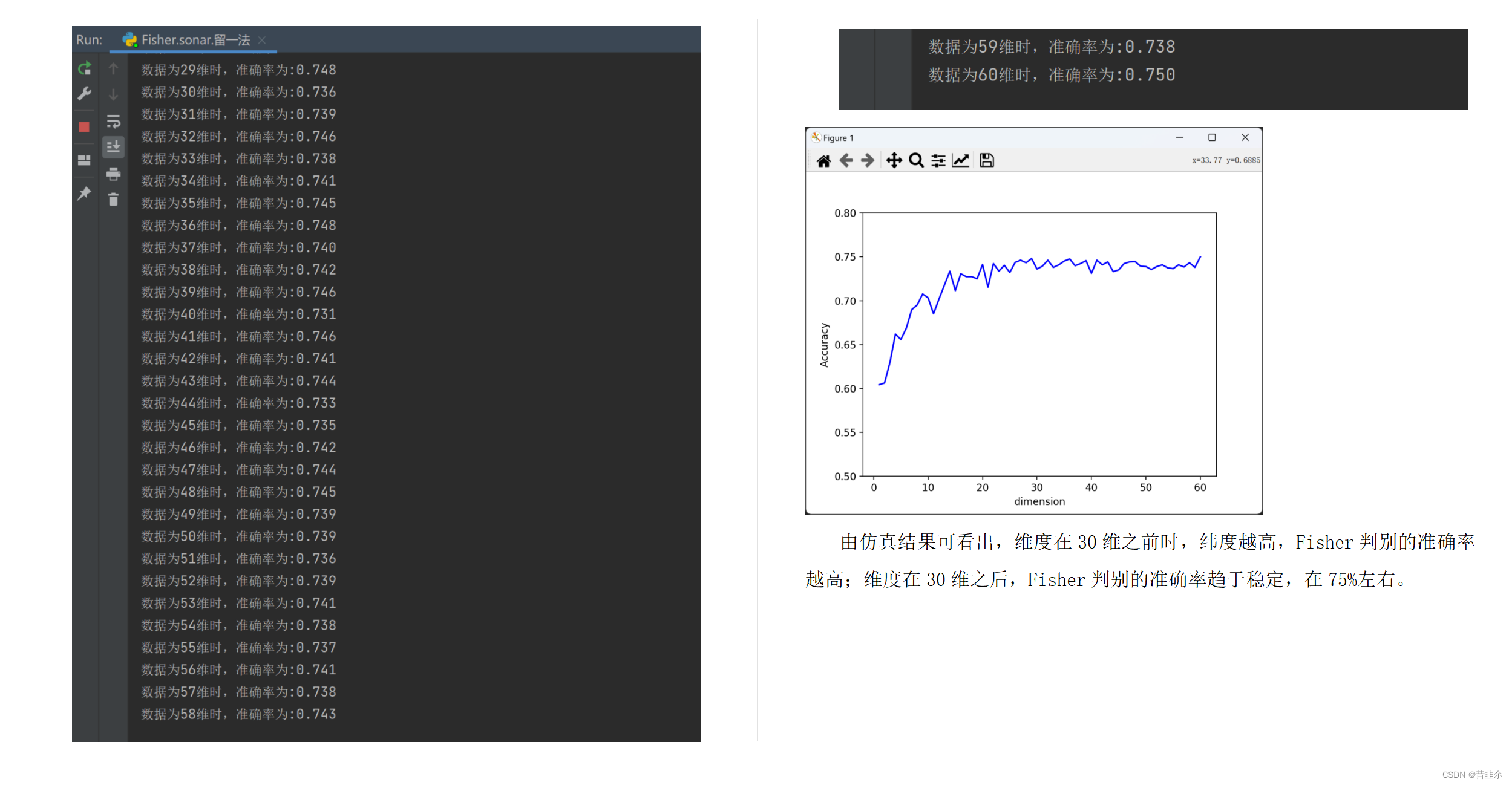
由仿真结果可看出，维度在30维之前时，纬度越高，Fisher判别的准确率越高；维度在30维之后，Fisher判别的准确率趋于稳定，在75%左右。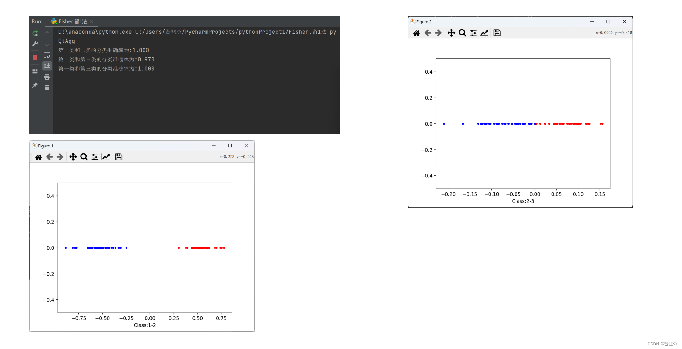

代码如下：

（1）iris数据集

import pandas as pd
import numpy as np
import matplotlib.pyplot as plt
import matplotlib as mpl
print(mpl.get_backend())Iris = pd.read_csv('iris.data', header=None, sep=',')def Fisher(X1, X2, t):# 各类样本均值向量m1 = np.mean(X1, axis=0)m2 = np.mean(X2, axis=0)m1 = m1.reshape(4, 1)m2 = m2.reshape(4, 1)m = m1 - m2# 样本类内离散度矩阵s1 = np.zeros((4, 4))   # s1,s2此时均为数组s2 = np.zeros((4, 4))if t == 0:  # 第一种情况for i in range(0, 49):s1 += (X1[i].reshape(4, 1) - m1).dot((X1[i].reshape(4, 1) - m1).T)for i in range(0, 50):s2 += (X2[i].reshape(4, 1) - m2).dot((X2[i].reshape(4, 1) - m2).T)if t == 1:  # 第二种情况for i in range(0, 50):s1 += (X1[i].reshape(4, 1) - m1).dot((X1[i].reshape(4, 1) - m1).T)for i in range(0, 49):s2 += (X2[i].reshape(4, 1) - m2).dot((X2[i].reshape(4, 1) - m2).T)# 总类内离散度矩阵sw = s1 + s2sw = np.mat(sw, dtype='float')m = np.mat(m, dtype='float')# 最佳投影方向w = np.linalg.inv(sw).dot(m)# 在投影后的一维空间求两类的均值m1 = np.mat(m1, dtype='float')m2 = np.mat(m2, dtype='float')m_1 = (w.T).dot(m1)m_2 = (w.T).dot(m2)# 计算分类阈值w0w0 = -0.5 * (m_1 + m_2)return w, w0def Classify(X,w,w0):y = (w.T).dot(X) + w0return y#数据预处理
Iris = Iris.iloc[0:150,0:4]
iris = np.mat(Iris)Accuracy = 0iris1 = iris[0:50, 0:4]
iris2 = iris[50:100, 0:4]
iris3 = iris[100:150, 0:4]G121 = np.ones(50)
G122 = np.ones(50)
G131 = np.zeros(50)
G132 = np.zeros(50)
G231 = np.zeros(50)
G232 = np.zeros(50)# 留一法验证准确性
# 第一类和第二类的线性判别
count = 0
for i in range(100):if i <= 49:test = iris1[i]test = test.reshape(4, 1)train = np.delete(iris1, i, axis=0)w, w0 = Fisher(train, iris2, 0)if (Classify(test, w, w0)) >= 0:count += 1G121[i] = Classify(test, w, w0)else:test = iris2[i-50]test = test.reshape(4, 1)train = np.delete(iris2, i-50, axis=0)w, w0 = Fisher(iris1, train, 1)if (Classify(test, w, w0)) < 0:count += 1G122[i-50] = Classify(test, w, w0)
Accuracy12 = count/100
print("第一类和二类的分类准确率为:%.3f"%(Accuracy12))# 第二类和第三类的线性判别
count = 0
for i in range(100):if i <= 49:test = iris2[i]test = test.reshape(4, 1)train = np.delete(iris2, i, axis=0)w, w0 = Fisher(train, iris3, 0)if (Classify(test, w, w0)) >= 0:count += 1G231[i] = Classify(test, w, w0)else:test = iris3[i-50]test = test.reshape(4, 1)train = np.delete(iris3, i-50, axis=0)w, w0 = Fisher(iris2, train, 1)if (Classify(test, w, w0)) < 0:count += 1G232[i-50] = Classify(test, w, w0)
Accuracy23 = count/100
print("第二类和第三类的分类准确率为:%.3f"%(Accuracy23))# 第一类和第三类的线性判别
count = 0
for i in range(100):if i <= 49:test = iris1[i]test = test.reshape(4, 1)train = np.delete(iris1, i, axis=0)w, w0 = Fisher(train, iris3, 0)if (Classify(test, w, w0)) >= 0:count += 1G131[i] = Classify(test, w, w0)else:test = iris3[i-50]test = test.reshape(4, 1)train = np.delete(iris3, i-50, axis=0)w,w0 = Fisher(iris1, train, 1)if (Classify(test, w, w0)) < 0:count += 1G132[i-50] = Classify(test, w, w0)
Accuracy13 = count/100
print("第一类和第三类的分类准确率为:%.3f"%(Accuracy13))# 作图
y1 = np.zeros(50)
y2 = np.zeros(50)
plt.figure(1)
plt.ylim((-0.5, 0.5))# 画散点图
plt.scatter(G121, y1, color='red', marker='.')
plt.scatter(G122, y2, color='blue', marker='.')
plt.xlabel('Class:1-2')
plt.show()plt.figure(2)
plt.ylim((-0.5, 0.5))
# 画散点图
plt.scatter(G231, y1, c='red',  marker='.')
plt.scatter(G232, y2, c='blue', marker='.')
plt.xlabel('Class:2-3')
plt.show()plt.figure(3)
plt.ylim((-0.5, 0.5))
# 画散点图
plt.scatter(G131, y1, c='red', marker='.')
plt.scatter(G132, y2, c='blue', marker='.')
plt.xlabel('Class:1-3')
plt.show()

（2）Sonar数据集

import numpy
import pandas as pd
import numpy as np
import matplotlib.pyplot as pltpath=r'sonar.all-data.txt'
df = pd.read_csv(path, header=None, sep=',')def Fisher(X1, X2, n, t):# 各类样本均值向量m1 = np.mean(X1, axis=0)m2 = np.mean(X2, axis=0)m1 = m1.reshape(n, 1)m2 = m2.reshape(n, 1)m = m1 - m2# 样本类内离散度矩阵s1 = np.zeros((n, n))   # s1,s2此时均为数组s2 = np.zeros((n, n))if t == 0:  # 第一种情况for i in range(0, 96):s1 += (X1[i].reshape(n, 1) - m1).dot((X1[i].reshape(n, 1) - m1).T)for i in range(0, 111):s2 += (X2[i].reshape(n, 1) - m2).dot((X2[i].reshape(n, 1) - m2).T)if t == 1:  # 第二种情况for i in range(0, 97):s1 += (X1[i].reshape(n, 1) - m1).dot((X1[i].reshape(n, 1) - m1).T)for i in range(0, 110):s2 += (X2[i].reshape(n, 1) - m2).dot((X2[i].reshape(n, 1) - m2).T)# 总类内离散度矩阵sw = s1 + s2sw = np.mat(sw, dtype='float')m = numpy.mat(m, dtype='float')# 最佳投影方向w = np.linalg.inv(sw).dot(m)# 在投影后的一维空间求两类的均值m_1 = (w.T).dot(m1)m_2 = (w.T).dot(m2)# 计算分类阈值w0w0 = -0.5 * (m_1 + m_2)return w, w0def Classify(X,w,w0):y = (w.T).dot(X) + w0return y# 数据预处理
Sonar = df.iloc[0:208,0:60]
sonar = np.mat(Sonar)# 分十次计算准确率
Accuracy = np.zeros(60)
accuracy_ = np.zeros(10)
for n in range(1,61):for t in range(10):sonar_random = (np.random.permutation(sonar.T)).T   # 对原sonar数据进行每列打乱sonar1 = sonar_random[0:97, 0:n]sonar2 = sonar_random[97:208, 0:n]count = 0# 留一法验证准确性for i in range(208):    # 取每一维度进行测试if i <= 96:test = sonar1[i]test = test.reshape(n, 1)train = np.delete(sonar1, i, axis=0)w, w0 = Fisher(train, sonar2, n, 0)if (Classify(test, w, w0)) >= 0:count += 1else:test = sonar2[i-97]test = test.reshape(n, 1)train = np.delete(sonar2, i-97, axis=0)w, w0 = Fisher(sonar1, train, n, 1)if (Classify(test, w, w0)) < 0:count += 1accuracy_[t] = count / 208for k in range(10):Accuracy[n - 1] += accuracy_[k]Accuracy[n - 1] = Accuracy[n - 1] / 10print("数据为%d维时，准确率为:%.3f" % (n, Accuracy[n - 1]))# 作图
x = np.arange(1, 61, 1)
plt.xlabel('dimension')
plt.ylabel('Accuracy')
plt.ylim((0.5, 0.8))            # y坐标的范围
plt.plot(x, Accuracy, 'b')
plt.show()