🔗 运行环境:Matlab
🚩 撰写作者:左手の明天
🥇 精选专栏:《python》
🔥 推荐专栏:《算法研究》
#### 防伪水印——左手の明天 ####
💗 大家好🤗🤗🤗,我是左手の明天!好久不见💗
💗今天开启新的系列——重新定义matlab强大系列💗
📆 最近更新:2023 年 09 月 24 日,左手の明天的第 292 篇原创博客
📚 更新于专栏:matlab
#### 防伪水印——左手の明天 ####
问题设立
假设有如下数据:
Data = ...[0.0000 5.89550.1000 3.56390.2000 2.51730.3000 1.97900.4000 1.89900.5000 1.39380.6000 1.13590.7000 1.00960.8000 1.03430.9000 0.84351.0000 0.68561.1000 0.61001.2000 0.53921.3000 0.39461.4000 0.39031.5000 0.54741.6000 0.34591.7000 0.13701.8000 0.22111.9000 0.17042.0000 0.2636];
利用matlab绘制这些数据点:
t = Data(:,1);
y = Data(:,2);
% axis([0 2 -0.5 6])
% hold on
plot(t,y,'ro')
title('Data points')
% hold off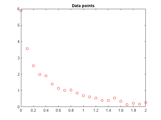
我们要对数据进行
y = c(1)*exp(-lam(1)*t) + c(2)*exp(-lam(2)*t)函数拟合。
使用 lsqcurvefit 的求解方法
lsqcurvefit 函数可以轻松求解这类问题。
首先,定义涉及一个变量 x 的参数:
x(1) = c(1)x(2) = lam(1)x(3) = c(2)x(4) = lam(2)然后将曲线定义为参数 x 和数据 t 的函数:
F = @(x,xdata)x(1)*exp(-x(2)*xdata) + x(3)*exp(-x(4)*xdata);任意设置一个初始点 x0 如下:c(1) = 1,lam(1) = 1,c(2) = 1,lam(2) = 0:
x0 = [1 1 1 0];运行求解器并绘制拟合结果。
[x,resnorm,~,exitflag,output] = lsqcurvefit(F,x0,t,y)Local minimum possible.lsqcurvefit stopped because the final change in the sum of squares relative to
its initial value is less than the value of the function tolerance.x = 1×43.0068   10.5869    2.8891    1.4003resnorm = 0.1477
exitflag = 3
output = struct with fields:firstorderopt: 7.8852e-06iterations: 6funcCount: 35cgiterations: 0algorithm: 'trust-region-reflective'stepsize: 0.0096message: 'Local minimum possible....'bestfeasible: []constrviolation: []
hold on
plot(t,F(x,t))
hold off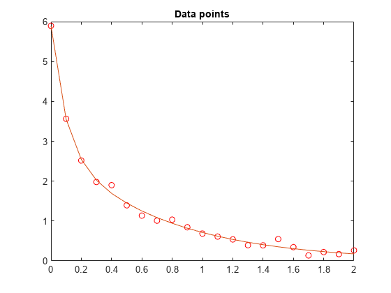
使用 fminunc 的求解方法
为了使用 fminunc 求解问题,将目标函数设置为残差的平方和。
Fsumsquares = @(x)sum((F(x,t) - y).^2);
opts = optimoptions('fminunc','Algorithm','quasi-newton');
[xunc,ressquared,eflag,outputu] = ...fminunc(Fsumsquares,x0,opts)
Local minimum found.Optimization completed because the size of the gradient is less than
the value of the optimality tolerance.
xunc = 1×42.8890    1.4003    3.0069   10.5862ressquared = 0.1477
eflag = 1
outputu = struct with fields:iterations: 30funcCount: 185stepsize: 0.0017lssteplength: 1firstorderopt: 2.9662e-05algorithm: 'quasi-newton'message: 'Local minimum found....'
请注意,fminunc 找到了与 lsqcurvefit 相同的解,但为此进行了更多的函数计算。fminunc 的参数与 lsqcurvefit 的参数顺序相反;较大的 lam 是 lam(2),而不是 lam(1)。这并不奇怪,变量的顺序是任意的。
fprintf(['There were %d iterations using fminunc,' ...' and %d using lsqcurvefit.\n'], ...outputu.iterations,output.iterations)There were 30 iterations using fminunc, and 6 using lsqcurvefit.fprintf(['There were %d function evaluations using fminunc,' ...' and %d using lsqcurvefit.'], ...outputu.funcCount,output.funcCount)There were 185 function evaluations using fminunc, and 35 using lsqcurvefit.拆分线性和非线性问题
请注意,拟合问题对于参数 c(1) 和 c(2) 是线性的。这意味着对于 lam(1) 和 lam(2) 的任何值,可以使用反斜杠运算符来找到求解最小二乘问题的 c(1) 和 c(2) 的值。
现在将此问题作为二维问题重新处理,搜索 lam(1) 和 lam(2) 的最佳值。在每步中按上面所述使用反斜杠运算符来计算 c(1) 和 c(2) 的值。
type fitvector
function yEst = fitvector(lam,xdata,ydata)
%FITVECTOR  Used by DATDEMO to return value of fitting function.
%   yEst = FITVECTOR(lam,xdata) returns the value of the fitting function, y
%   (defined below), at the data points xdata with parameters set to lam.
%   yEst is returned as a N-by-1 column vector, where N is the number of
%   data points.
%
%   FITVECTOR assumes the fitting function, y, takes the form
%
%     y =  c(1)*exp(-lam(1)*t) + ... + c(n)*exp(-lam(n)*t)
%
%   with n linear parameters c, and n nonlinear parameters lam.
%
%   To solve for the linear parameters c, we build a matrix A
%   where the j-th column of A is exp(-lam(j)*xdata) (xdata is a vector).
%   Then we solve A*c = ydata for the linear least-squares solution c,
%   where ydata is the observed values of y.A = zeros(length(xdata),length(lam));  % build A matrix
for j = 1:length(lam)A(:,j) = exp(-lam(j)*xdata);
end
c = A\ydata; % solve A*c = y for linear parameters c
yEst = A*c; % return the estimated response based on c
使用 lsqcurvefit 求解问题,从二维初始点 lam(1), lam(2) 开始:
x02 = [1 0];
F2 = @(x,t) fitvector(x,t,y);[x2,resnorm2,~,exitflag2,output2] = lsqcurvefit(F2,x02,t,y)
Local minimum possible.lsqcurvefit stopped because the final change in the sum of squares relative to
its initial value is less than the value of the function tolerance.
x2 = 1×210.5861    1.4003resnorm2 = 0.1477
exitflag2 = 3
output2 = struct with fields:firstorderopt: 4.4018e-06iterations: 10funcCount: 33cgiterations: 0algorithm: 'trust-region-reflective'stepsize: 0.0080message: 'Local minimum possible....'bestfeasible: []constrviolation: []
二维求解的效率类似于四维求解的效率:
fprintf(['There were %d function evaluations using the 2-d ' ...'formulation, and %d using the 4-d formulation.'], ...output2.funcCount,output.funcCount)There were 33 function evaluations using the 2-d formulation, and 35 using the 4-d formulation.对于初始估计值来说,拆分问题更稳健
为最初的四参数问题选择的起点不理想会得到局部解,而非全局解。为拆分的两参数问题选择具有同样不理想的 lam(1) 和 lam(2) 值的起点会得到全局解。为了说明这一点,使用会得到相对较差的局部解的起点重新运行原始问题,并将得到的拟合与全局解进行比较。
线性拟合
多项式拟合
多项式拟合就是利用下面形式的方程去拟合数据:

matlab中可以用polyfit()函数进行多项式拟合。
polyfit-多项式曲线拟合
p = polyfit(x,y,n) 返回次数为 n 的多项式 p(x) 的系数,该阶数是 y 中数据的最佳拟合(基于最小二乘指标)。p 中的系数按降幂排列,p 的长度为 n+1
![]()
将多项式与三角函数拟合
在区间 [0,4*pi] 中沿正弦曲线生成 10 个等间距的点。
x = linspace(0,4*pi,10);
y = sin(x);
使用 polyfit 将一个 7 次多项式与这些点拟合。
p = polyfit(x,y,7);在更精细的网格上计算多项式并绘制结果图。
x1 = linspace(0,4*pi);
y1 = polyval(p,x1);
figure
plot(x,y,'o')
hold on
plot(x1,y1)
hold off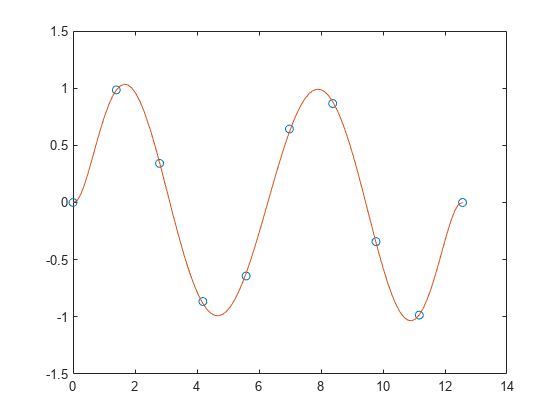
将多项式与点集拟合
创建一个由区间 [0,1] 中的 5 个等间距点组成的向量,并计算这些点处的 y(x)=(1+x)−1。
x = linspace(0,1,5);
y = 1./(1+x);
将 4 次多项式与 5 个点拟合。通常,对于 n 个点,可以拟合 n-1 次多项式以便完全通过这些点。
p = polyfit(x,y,4);在由 0 和 2 之间的点组成的更精细网格上计算原始函数和多项式拟合。
x1 = linspace(0,2);
y1 = 1./(1+x1);
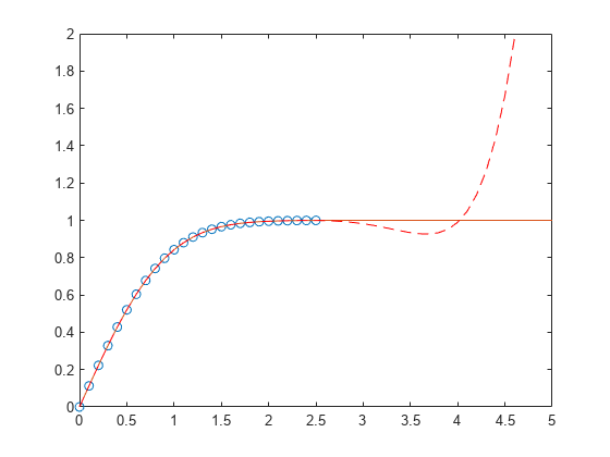
f1 = polyval(p,x1);在更大的区间 [0,2] 中绘制函数值和多项式拟合,其中包含用于获取以圆形突出显示的多项式拟合的点。多项式拟合在原始 [0,1] 区间中的效果较好,但在该区间外部很快与拟合函数出现差异。
figure
plot(x,y,'o')
hold on
plot(x1,y1)
plot(x1,f1,'r--')
legend('y','y1','f1')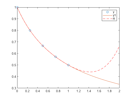
对误差函数进行多项式拟合
首先生成 x 点的向量,在区间 [0,2.5] 内等间距分布;然后计算这些点处的 erf(x)。
x = (0:0.1:2.5)';
y = erf(x);
确定 6 次逼近多项式的系数。
p = polyfit(x,y,6)p = 1×70.0084 -0.0983 0.4217 -0.7435 0.1471 1.1064 0.0004
为了查看拟合情况如何,在各数据点处计算多项式,并生成说明数据、拟合和误差的一个表。
f = polyval(p,x);
T = table(x,y,f,y-f,'VariableNames',{'X','Y','Fit','FitError'})T=26×4 tableX        Y          Fit         FitError  ___    _______    __________    ___________0          0    0.00044117    -0.000441170.1    0.11246       0.11185     0.000608360.2     0.2227       0.22231     0.000391890.3    0.32863       0.32872    -9.7429e-050.4    0.42839        0.4288    -0.000406610.5     0.5205       0.52093    -0.000425680.6    0.60386       0.60408    -0.000228240.7     0.6778       0.67775     4.6383e-050.8     0.7421       0.74183     0.000269920.9    0.79691       0.79654     0.000365151     0.8427       0.84238      0.00031641.1    0.88021       0.88005     0.000159481.2    0.91031       0.91035    -3.9919e-051.3    0.93401       0.93422      -0.0002111.4    0.95229       0.95258    -0.000299331.5    0.96611       0.96639    -0.00028097⋮
在该区间中,插值与实际值非常符合。创建
x1 = (0:0.1:5)';
y1 = erf(x1);
f1 = polyval(p,x1);
figure
plot(x,y,'o')
hold on
plot(x1,y1,'-')
plot(x1,f1,'r--')
axis([0  5  0  2])
hold off
一个绘图,以显示在该区间以外,外插值与实际数据值如何快速偏离。
简单线性回归
将一个简单线性回归模型与一组离散二维数据点拟合。
创建几个由样本数据点 (x,y) 组成的向量。对数据进行一次多项式拟合。
x = 1:50;
y = -0.3*x + 2*randn(1,50);
p = polyfit(x,y,1);
计算在 x 中的点处拟合的多项式 p。用这些数据绘制得到的线性回归模型。
f = polyval(p,x);
plot(x,y,'o',x,f,'-')
legend('data','linear fit') 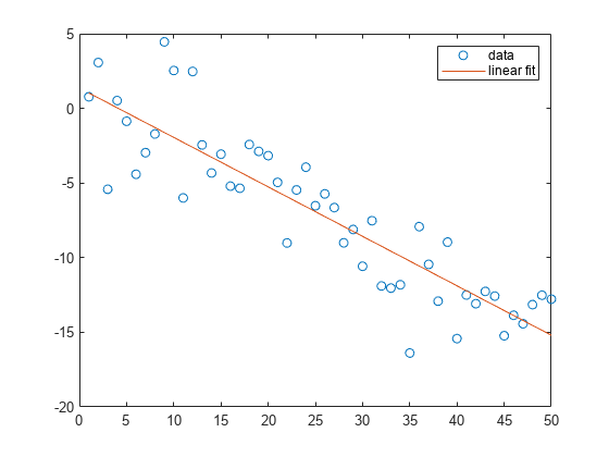
具有误差估计值的线性回归
将一个线性模型拟合到一组数据点并绘制结果,其中包含预测区间为 95% 的估计值。
创建几个由样本数据点 (x,y) 组成的向量。使用 polyfit 对数据进行一次多项式拟合。指定两个输出以返回线性拟合的系数以及误差估计结构体。
x = 1:100;
y = -0.3*x + 2*randn(1,100);
[p,S] = polyfit(x,y,1);
计算以 p 为系数的一次多项式在 x 中各点处的拟合值。将误差估计结构体指定为第三个输入,以便 polyval 计算标准误差的估计值。标准误差估计值在 delta 中返回。
[y_fit,delta] = polyval(p,x,S);绘制原始数据、线性拟合和 95% 预测区间 y±2Δ。
plot(x,y,'bo')
hold on
plot(x,y_fit,'r-')
plot(x,y_fit+2*delta,'m--',x,y_fit-2*delta,'m--')
title('Linear Fit of Data with 95% Prediction Interval')
legend('Data','Linear Fit','95% Prediction Interval')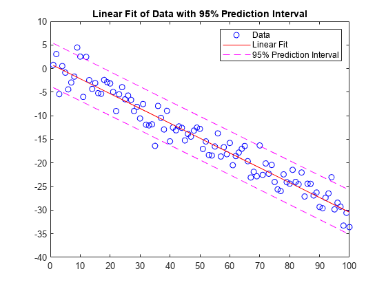
对于多项式拟合,不是阶数越多越好。比如看以下例子,阶数越多,曲线越能够穿过每一个点,但是曲线的形状与理论曲线偏离越大。所以选择最适合的才是最好的。
x=0:0.5:10;
y=0.03*x.^4-0.5*x.^3+2.0*x.^2-0*x-4+6*(rand(size(x))-0.5);
p=polyfit(x,y,4);
x2=0:0.05:10;
y2=polyval(p,x2);
figure();
subplot(1,2,1)
hold on
plot(x,y,'linewidth',1.5,'MarkerSize',15,'Marker','.','color','k')
plot(x,0.03*x.^4-0.5*x.^3+2.0*x.^2-0*x-4,'linewidth',1,'color','b')
hold off
legend('原始数据点','理论曲线','Location','southoutside','Orientation','horizontal')
legend('boxoff')
box on
subplot(1,2,2)
hold on
plot(x2,y2,'-','linewidth',1.5,'color','r')
plot(x,y,'LineStyle','none','MarkerSize',15,'Marker','.','color','k')
hold off
box on
legend('拟合曲线','数据点','Location','southoutside','Orientation','horizontal')
legend('boxoff')
线性拟合
线性拟合就是能够把拟合函数写成下面这种形式的:

其中f(x)是关于x的函数,其表达式是已知的。p是常数系数,这个是未知的。
举个例子

虽然看上去很非线性,但是x和y都是已知的,a、b、c是未知的,而且是线性的,所以可以被非常简单的拟合出来。假设a=2.5,b=0.5,c=-1,加入随机扰动。
x=0:0.5:10;
a=2.5;
b=0.5;
c=-1;y=a*sin(0.2*x.^2+x)+b*sqrt(x+1)+c+0.5*rand(size(x));yn1=sin(0.2*x.^2+x);
yn2=sqrt(x+1);
yn3=ones(size(x));
X=[yn1;yn2;yn3];Pn=X'\y';
yn=Pn(1)*yn1+Pn(2)*yn2+Pn(3)*yn3;figure()
subplot(1,2,1)
plot(x,y,'linewidth',1.5,'MarkerSize',15,'Marker','.','color','k')
legend('原始数据点','Location','southoutside','Orientation','horizontal')
legend('boxoff')
subplot(1,2,2)
hold on
x2=0:0.01:10;
plot(x2,Pn(1)*sin(0.2*x2.^2+x2)+Pn(2)*sqrt(x2+1)+Pn(3),'-','linewidth',1.5,'color','r')
plot(x,y,'LineStyle','none','MarkerSize',15,'Marker','.','color','k')
hold off
box on
legend('拟合曲线','数据点','Location','southoutside','Orientation','horizontal')
legend('boxoff')
拟合的最终效果为:

最终得到的拟合参数为:a=2.47,b=0.47,c=-0.66。