目录
一、实验内容
二、实验过程
2.1.1 test.py文件
2.1.2 test.py文件结果与分析
2.2.1 文件代码
2.2.2 结果与分析
一、实验内容
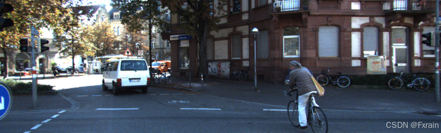
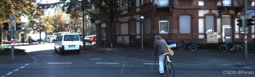
- 给定左右相机图片,估算图片的视差/深度;体现极线校正(例如打印前后极线对)、同名点匹配(例如打印数量、或可视化部分匹配点)、估计结果(部分像素的视差或深度)。
- 评估基线长短、不同场景(室内、室外)对算法的影响。
二、实验过程
2.1.1 test.py文件
from PIL import Image
from pylab import *
from scipy.ndimage import *
import numpy as np
import cv2
import matplotlib.pyplot as plt
from scipy.ndimage import filtersdef plane_sweep_ncc(im_l, im_r, start, steps, wid):m, n = im_l.shapemean_l = np.zeros((m, n))mean_r = np.zeros((m, n))s = np.zeros((m, n))s_l = np.zeros((m, n))s_r = np.zeros((m, n))dmaps = np.zeros((m, n, steps))filters.uniform_filter(im_l, wid, mean_l)filters.uniform_filter(im_r, wid, mean_r)norm_l = im_l - mean_lnorm_r = im_r - mean_rfor displ in range(steps):filters.uniform_filter(np.roll(norm_l, -displ - start) * norm_r, wid, s)filters.uniform_filter(np.roll(norm_l, -displ - start) * np.roll(norm_l, -displ - start), wid, s_l)filters.uniform_filter(norm_r * norm_r, wid, s_r)with np.errstate(invalid='ignore'):denominator = np.sqrt(s_l * s_r)denominator[denominator == 0] = np.inf dmaps[:, :, displ] = s / denominatorreturn np.argmax(dmaps, axis=2)def epipolar_correction(im_l, im_r, F):h, w = im_l.shapecorrected_r = np.zeros_like(im_r)for y in range(h):for x in range(w):pt = np.array([x, y, 1])line = F @ ptline = line / line[0]a, b, c = lineu = int(round(-c / a))v = int(round(-c / b))if 0 <= u < w and 0 <= v < h:corrected_r[y, x] = im_r[v, u]print(f"\n校正前位置坐标: ({x}, {y}) -> 校正后位置坐标: ({u}, {v})")return corrected_rdef find_matches(im_l, im_r):sift = cv2.SIFT_create()kp1, des1 = sift.detectAndCompute(im_l.astype(np.uint8), None)kp2, des2 = sift.detectAndCompute(im_r.astype(np.uint8), None)bf = cv2.BFMatcher()matches = bf.knnMatch(des1, des2, k=2)good_matches = []for m, n in matches:if m.distance < 0.75 * n.distance:good_matches.append(m)return kp1, kp2, good_matchesdef compute_fundamental_matrix(kp1, kp2, matches):points1 = np.float32([kp1[m.queryIdx].pt for m in matches])points2 = np.float32([kp2[m.trainIdx].pt for m in matches])F, mask = cv2.findFundamentalMat(points1, points2, cv2.FM_RANSAC)return Fdef visualize_results(im_l, im_r, im_r_corrected, kp1, kp2, matches):fig, axs = plt.subplots(1, 3, figsize=(15, 5))axs[0].imshow(im_l, cmap='gray')axs[0].set_title('Left Image')axs[0].axis('off')axs[1].imshow(im_r, cmap='gray')axs[1].set_title('Right Image')axs[1].axis('off')axs[2].imshow(im_r_corrected, cmap='gray')axs[2].set_title('Corrected Right Image')axs[2].axis('off')plt.show()img_matches = cv2.drawMatches(im_l.astype(np.uint8), kp1, im_r.astype(np.uint8), kp2, matches[:10], None, flags=cv2.DrawMatchesFlags_NOT_DRAW_SINGLE_POINTS)plt.figure(figsize=(10, 5))plt.imshow(img_matches)plt.title('Top 10 Matches')plt.axis('off')plt.show()im_l = np.array(Image.open('D:\\Computer vision\\KITTI2015_part\\left\\000000_10.png').convert('L'), 'f')
im_r = np.array(Image.open('D:\\Computer vision\\KITTI2015_part\\right\\000000_10.png').convert('L'), 'f')
steps = 50
start = 4
wid = 13kp1, kp2, matches = find_matches(im_l, im_r)
F = compute_fundamental_matrix(kp1, kp2, matches)im_r_corrected = epipolar_correction(im_l, im_r, F)
visualize_results(im_l, im_r, im_r_corrected, kp1, kp2, matches)
res = plane_sweep_ncc(im_l, im_r_corrected, start, steps, wid)
imsave('D:\\Computer vision\\KITTI2015_part\\12_3test.jpg', res)
2.1.2 test.py文件结果与分析
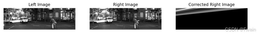
上述代码通过特征点检测、基础矩阵计算、极线校正以及视差图计算实现了立体匹配和校正的流程。
结果一:
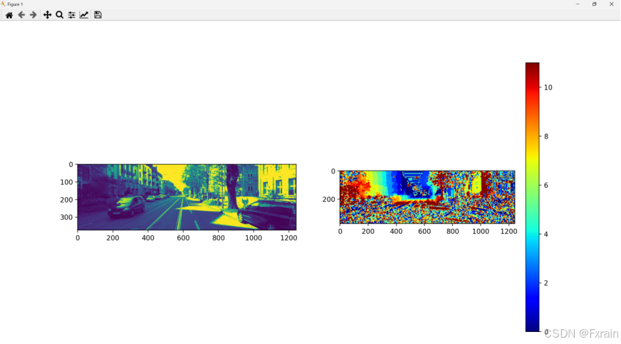
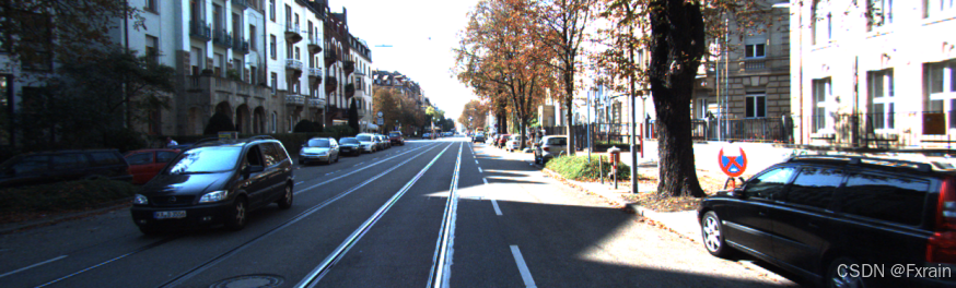
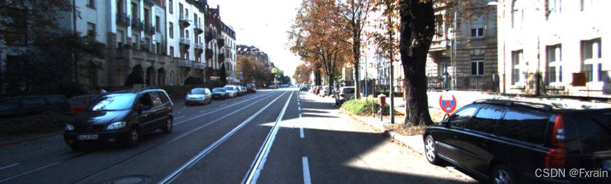
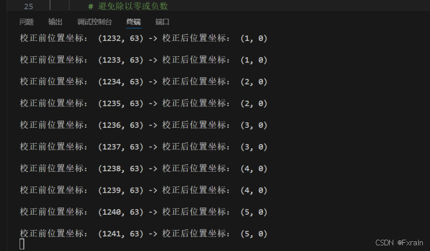
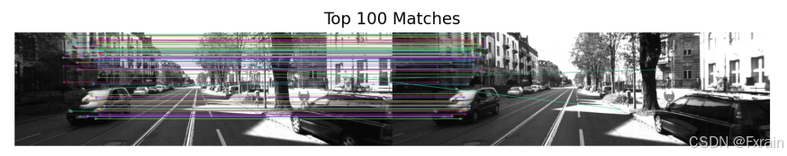
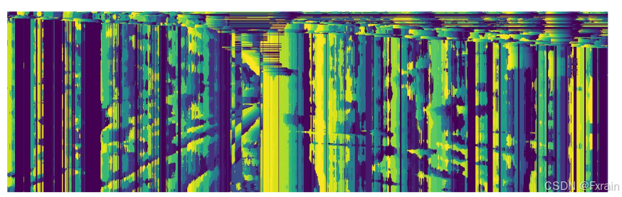
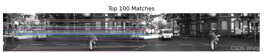
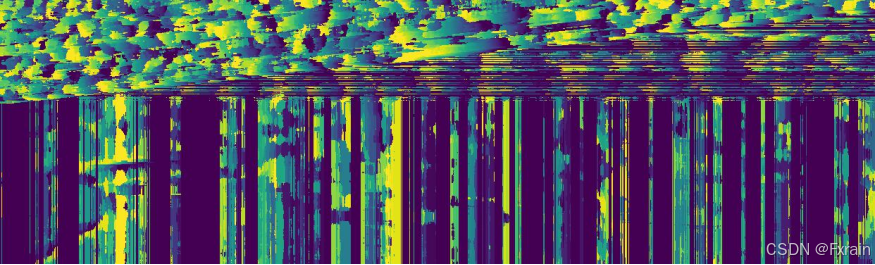
数据集如下图图1、图2所示,图3展示了极线校正前后坐标信息的部分截图,图4展示了部分同名点匹配结果,图5展示了视差估计结果。
结果二:
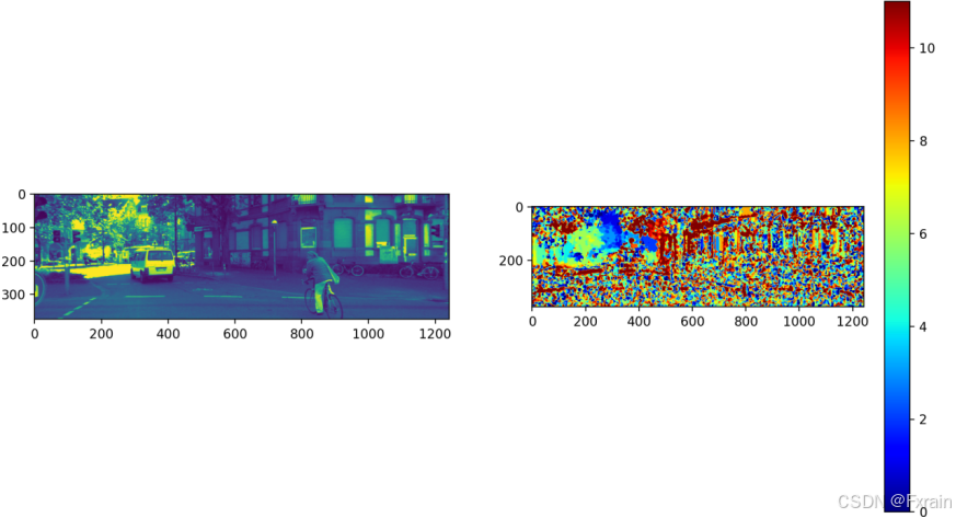
数据集如下图图6、图7所示,图8展示了极线校正前后坐标信息的部分截图,图9展示了部分同名点匹配结果,图10展示了视差估计结果。
2.2.1 文件代码
a.stereo_module.py文件
from numpy import argmax, roll, sqrt, zeros
from scipy.ndimage import filters
def plane_sweep_ncc(im_l,im_r,start,steps,wid):m,n=im_l.shapemean_l=zeros((m,n))mean_r=zeros((m,n))s=zeros((m,n))s_l=zeros((m,n))s_r=zeros((m,n))dmaps=zeros((m,n,steps))filters.uniform_filter(im_l,wid,mean_l)filters.uniform_filter(im_r,wid,mean_r)norm_l=im_l-mean_lnorm_r=im_r-mean_rfor displ in range(steps):filters.uniform_filter(roll(norm_l,-displ-start)*norm_r,wid,s)filters.uniform_filter(roll(norm_l,-displ-start)*roll(norm_l,-displ-start),wid,s_l)filters.uniform_filter(norm_r*norm_r,wid,s_r)dmaps[:,:,displ]=s/sqrt(s_l*s_r)return argmax(dmaps,axis=2)def plane_sweep_gauss(im_l,im_r,start,steps,wid):m,n = im_l.shape# arrays to hold the different sumsmean_l = zeros((m,n))mean_r = zeros((m,n))s = zeros((m,n))s_l = zeros((m,n))s_r = zeros((m,n))dmaps = zeros((m,n,steps))filters.gaussian_filter(im_l,wid,0,mean_l)filters.gaussian_filter(im_r,wid,0,mean_r)norm_l = im_l - mean_lnorm_r = im_r - mean_rfor displ in range(steps):filters.gaussian_filter(roll(norm_l,-displ-start)*norm_r,wid,0,s) filters.gaussian_filter(roll(norm_l,-displ-start)*roll(norm_l,-displ-start),wid,0,s_l)filters.gaussian_filter(norm_r*norm_r,wid,0,s_r) dmaps[:,:,displ] = s/sqrt(s_l*s_r)return argmax(dmaps,axis=2)
b. stereo_test.py文件
from matplotlib import colorbar
from matplotlib.pyplot import imshow, show, subplot
from numpy import array
from PIL import Image
import stereo_module as stereo
import cv2
import matplotlib.pyplot as plt
im_l=array(Image.open('D:\\Computer vision\\KITTI2015_part\\left\\000000_10.png').convert('L'),'f')
im_r=array(Image.open('D:\Computer vision\\KITTI2015_part\\right\\000000_10.png').convert('L'),'f')
steps=12
start=4
wid=9
res_ncc=stereo.plane_sweep_ncc(im_l,im_r,start,steps,wid)
cv2.imwrite('D:\\Computer vision\\KITTI2015_part\\depth_ncc.png',res_ncc)
res_gauss=stereo.plane_sweep_gauss(im_l,im_r,start,steps,wid)
cv2.imwrite('D:\\Computer vision\\KITTI2015_part\\depth_gauss.png',res_gauss)subplot(121)
imshow(im_l)subplot(122)
imshow(res_ncc, cmap='jet')
plt.colorbar()
show()
2.2.2 结果与分析
视差估计结果如图11、图12所示