经纬度聚类：聚类算法比较

需求：

将经纬度数据，根据经纬度进行聚类

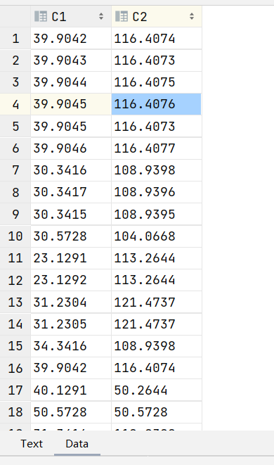
初始数据

data.csv

K均值聚类

简介

K均值（K-means）聚类是一种常用的无监督学习算法，用于将数据集中的样本分成K个不同的簇（cluster）。其基本思想是将数据集划分为K个簇，使得每个样本点都属于距离最近的簇的中心点，同时最小化簇内样本点之间的距离平方和。

K均值聚类算法的步骤如下：

初始化: 随机选择K个样本点作为初始的簇中心点。
分配: 对于每个样本点，计算其与K个簇中心点的距离，并将其分配到距离最近的簇中心点所在的簇。
更新: 对于每个簇，计算其所有样本点的均值，将该均值作为新的簇中心点。
重复迭代: 重复步骤2和步骤3，直到簇中心点不再发生变化或达到预设的迭代次数。

优点

简单易实现、计算速度快

缺点

对初始聚类中心点敏感、对异常值敏感，在实际应用中，通常需要进行多次运行并选择最优的聚类结果。

使用场景

适用于数据集没有明确标签信息、簇形状相对简单、簇大小相近的情况下，常用于图像压缩、文本聚类、客户分群等领域。

簇个数已知：K均值聚类需要预先指定簇的个数，因此适用于已知簇个数的情况。
数据集各个簇的形状相似：K均值聚类假设每个簇是凸形的，且具有相似的大小和密度，因此适用于各个簇形状相似的数据集。
对速度要求高：K均值聚类是一种简单且高效的算法，适用于大规模数据集和对速度要求高的场景。
聚类结果可解释性强：K均值聚类产生的簇中心代表了每个簇的平均特征，因此聚类结果具有较强的可解释性，适用于需要直观理解聚类结果的场景。
数据特征空间是欧几里得空间：K均值聚类使用欧几里得距离来度量数据点之间的相似度，因此适用于特征空间是欧几里得空间的情况。
初始中心点的选择相对灵活：虽然K均值聚类对初始中心点的选择敏感，但是可以采用多次随机初始化来减少此影响，因此对于初始中心点的选择相对灵活。

java代码实现

public class KMeansClustering {// 加载数据public static List<Point> loadData(String filename) {List<Point> points = new ArrayList<>();try (BufferedReader br = new BufferedReader(new FileReader(filename))) {String line;while ((line = br.readLine()) != null) {String[] parts = line.split(",");double latitude = Double.parseDouble(parts[0]);double longitude = Double.parseDouble(parts[1]);points.add(new Point(latitude, longitude));}} catch (IOException e) {e.printStackTrace();}return points;}private int k; // 聚类数量private List<Point> centroids; // 聚类中心点public KMeansClustering(int k) {this.k = k;this.centroids = new ArrayList<>();}// 初始化聚类中心点private void initCentroids(List<Point> points) {Random random = new Random();for (int i = 0; i < k; i++) {Point centroid = points.get(random.nextInt(points.size()));centroids.add(centroid);}}// 计算两点之间的欧氏距离private double calculateDistance(Point a, Point b) {return Math.sqrt(Math.pow(a.getX() - b.getX(), 2) + Math.pow(a.getY() - b.getY(), 2));}/*** 执行K均值聚类算法。** @param points 含有点的列表，每个点包含x和y坐标。* @param maxIterations 最大迭代次数。* @return 返回包含点的聚类列表，每个聚类是一个包含点的列表。*/public List<List<Point>> kMeans(List<Point> points, int maxIterations) {// 初始化聚类中心点initCentroids(points);List<List<Point>> clusters = new ArrayList<>();for (int i = 0; i < maxIterations; i++) {clusters.clear();// 初始化簇for (int j = 0; j < k; j++) {clusters.add(new ArrayList<>());}// 分配点到最近的簇for (Point point : points) {double minDistance = Double.MAX_VALUE;int closestCentroidIndex = -1;// 计算点到各个聚类中心的距离，分配点到最近的聚类中心for (int j = 0; j < k; j++) {double distance = calculateDistance(point, centroids.get(j));if (distance < minDistance) {minDistance = distance;closestCentroidIndex = j;}}clusters.get(closestCentroidIndex).add(point);}// 更新聚类中心点for (int j = 0; j < k; j++) {List<Point> cluster = clusters.get(j);double sumX = 0, sumY = 0;// 计算聚类中心for (Point point : cluster) {sumX += point.getX();sumY += point.getY();}centroids.set(j, new Point(sumX / cluster.size(), sumY / cluster.size()));}}return clusters;}public static void main(String[] args) {// 读取数据文件String inputFile = "data.csv";List<Point> points = loadData(inputFile);long l = System.currentTimeMillis();KMeansClustering kMeans = new KMeansClustering(4); // 聚类数量为4List<List<Point>> clusters = kMeans.kMeans(points, 1000); // 最大迭代次数为10// 输出聚类结果for (int i = 0; i < clusters.size(); i++) {System.out.println("聚类 " + (i + 1) + ":");for (Point point : clusters.get(i)) {System.out.println("(" + point.getX() + ", " + point.getY() + ")");}System.out.println();}System.out.println("耗时：" + (System.currentTimeMillis() - l) + "ms");}
}class Point {private double x;private double y;public Point(double x, double y) {this.x = x;this.y = y;}public double getX() {return x;}public double getY() {return y;}
}

输出结果

第一次

聚类 1:
(12.9042, 12.4074)
(32.1291, 32.2644)
(21.2304, 21.4737)
(15.1291, 16.2644)
(23.1281, 56.2644)
(23.5728, 43.0668)
(21.3416, 32.9398)
(33.1291, 33.1291)
(12.2304, 43.4737)
(34.5728, 43.0668)
(34.3416, 34.9398)
(23.1291, 65.2644)
(30.5728, 21.0668)
(34.3416, 21.9398)
(21.9042, 32.4074)
(23.2304, 43.4737)
(23.1291, 34.2643)聚类 2:
(30.3416, 108.9398)
(30.3417, 108.9396)
(30.3415, 108.9395)
(30.5728, 104.0668)
(23.1291, 113.2644)
(23.1292, 113.2644)
(23.1292, 113.1232)
(30.121, 104.2121)
(32.3416, 104.2132)
(42.2304, 92.4736)
(33.3416, 89.9398)
(21.9042, 89.4074)
(21.5728, 104.0666)
(12.3416, 76.9398)
(14.9042, 78.4074)
(23.3416, 108.9398)聚类 3:
(40.1291, 50.2644)
(50.5728, 50.5728)
(43.2304, 41.4737)
(45.5728, 43.0668)
(65.5727, 65.0623)
(76.9042, 54.4074)
(45.2304, 65.4737)
(66.5728, 31.0668)
(31.2304, 65.4737)
(56.5728, 67.0668)
(67.2304, 32.4737)聚类 4:
(39.9042, 116.4074)
(39.9043, 116.4073)
(39.9044, 116.4075)
(39.9045, 116.4076)
(39.9045, 116.4073)
(39.9046, 116.4077)
(31.2304, 121.4737)
(31.2305, 121.4737)
(34.3416, 108.9398)
(39.9042, 116.4074)
(31.3416, 118.9398)
(39.9042, 116.4074)
(39.904, 116.4071)
(65.9042, 116.4074)
(34.9042, 116.4074)
(53.1291, 113.2645)耗时：37ms

第二次

聚类 1:
(40.1291, 50.2644)
(12.9042, 12.4074)
(43.2304, 41.4737)
(32.1291, 32.2644)
(21.2304, 21.4737)
(15.1291, 16.2644)
(23.1281, 56.2644)
(23.5728, 43.0668)
(21.3416, 32.9398)
(33.1291, 33.1291)
(12.2304, 43.4737)
(34.5728, 43.0668)
(34.3416, 34.9398)
(31.2304, 65.4737)
(23.1291, 65.2644)
(30.5728, 21.0668)
(34.3416, 21.9398)
(21.9042, 32.4074)
(23.2304, 43.4737)
(23.1291, 34.2643)聚类 2:
(50.5728, 50.5728)
(45.5728, 43.0668)
(65.5727, 65.0623)
(76.9042, 54.4074)
(45.2304, 65.4737)
(66.5728, 31.0668)
(56.5728, 67.0668)
(67.2304, 32.4737)聚类 3:
(30.3416, 108.9398)
(30.3417, 108.9396)
(30.3415, 108.9395)
(30.5728, 104.0668)
(23.1291, 113.2644)
(23.1292, 113.2644)
(23.1292, 113.1232)
(30.121, 104.2121)
(32.3416, 104.2132)
(42.2304, 92.4736)
(33.3416, 89.9398)
(21.9042, 89.4074)
(21.5728, 104.0666)
(12.3416, 76.9398)
(14.9042, 78.4074)
(23.3416, 108.9398)聚类 4:
(39.9042, 116.4074)
(39.9043, 116.4073)
(39.9044, 116.4075)
(39.9045, 116.4076)
(39.9045, 116.4073)
(39.9046, 116.4077)
(31.2304, 121.4737)
(31.2305, 121.4737)
(34.3416, 108.9398)
(39.9042, 116.4074)
(31.3416, 118.9398)
(39.9042, 116.4074)
(39.904, 116.4071)
(65.9042, 116.4074)
(34.9042, 116.4074)
(53.1291, 113.2645)耗时：50ms

第三次

聚类 1:
(12.9042, 12.4074)
(32.1291, 32.2644)
(21.2304, 21.4737)
(15.1291, 16.2644)
(23.5728, 43.0668)
(21.3416, 32.9398)
(33.1291, 33.1291)
(12.2304, 43.4737)
(34.5728, 43.0668)
(34.3416, 34.9398)
(30.5728, 21.0668)
(34.3416, 21.9398)
(21.9042, 32.4074)
(23.2304, 43.4737)
(23.1291, 34.2643)聚类 2:
(39.9042, 116.4074)
(39.9043, 116.4073)
(39.9044, 116.4075)
(39.9045, 116.4076)
(39.9045, 116.4073)
(39.9046, 116.4077)
(30.3416, 108.9398)
(30.3417, 108.9396)
(30.3415, 108.9395)
(30.5728, 104.0668)
(23.1291, 113.2644)
(23.1292, 113.2644)
(31.2304, 121.4737)
(31.2305, 121.4737)
(34.3416, 108.9398)
(39.9042, 116.4074)
(31.3416, 118.9398)
(39.9042, 116.4074)
(39.904, 116.4071)
(23.1292, 113.1232)
(30.121, 104.2121)
(32.3416, 104.2132)
(42.2304, 92.4736)
(21.5728, 104.0666)
(65.9042, 116.4074)
(23.3416, 108.9398)
(34.9042, 116.4074)
(53.1291, 113.2645)聚类 3:
(40.1291, 50.2644)
(50.5728, 50.5728)
(43.2304, 41.4737)
(45.5728, 43.0668)
(65.5727, 65.0623)
(76.9042, 54.4074)
(45.2304, 65.4737)
(66.5728, 31.0668)
(56.5728, 67.0668)
(67.2304, 32.4737)聚类 4:
(33.3416, 89.9398)
(21.9042, 89.4074)
(23.1281, 56.2644)
(12.3416, 76.9398)
(14.9042, 78.4074)
(31.2304, 65.4737)
(23.1291, 65.2644)耗时：50ms

结论：不适合此需求

可见，K均值聚类算法的每次输出的结果并不一致，输出结果不稳定。对初始聚类中心点敏感、对异常值敏感，而且不会剔除干扰点，K均值聚类算法会将所有结果进行分组聚类。

DBSCAN聚类 算法

简介

DBSCAN（Density-Based Spatial Clustering of Applications with Noise）是一种基于密度的聚类算法，能够发现任意形状的簇，并且能够有效处理数据中的噪声点。与K均值聚类不同，DBSCAN不需要提前指定簇的个数，而是根据数据的密度来确定簇的形状和数量。

DBSCAN算法的主要思想是以数据点的密度为基础，通过以下两个参数来定义：

ε（eps）: 邻域半径，用于确定一个点的邻域范围。
MinPts: 邻域内最少点数，用于判断一个点是否为核心点。

基于这两个参数，DBSCAN将数据点分为三类：

核心点（Core Point）: 在其ε邻域内包含至少MinPts个点的数据点。
边界点（Border Point）: 不是核心点，但位于核心点的ε邻域内。
噪声点（Noise Point）: 既不是核心点也不是边界点的数据点。

DBSCAN算法的步骤如下：

初始化: 随机选择一个未被访问的数据点。
密度可达性查询: 判断该点是否为核心点，如果是核心点，则将其加入一个新的簇，同时通过密度可达性查询将该簇中所有密度可达的点加入簇中。
重复步骤2: 直到所有的数据点都被访问过。

优点

能够自动发现任意形状的簇、对噪声点具有鲁棒性等

缺点

DBSCAN的性能会受到ε和MinPts参数的影响，需要谨慎选择这两个参数。

使用场景

发现任意形状的簇：DBSCAN不需要预先指定簇的个数，并且能够自动识别不规则形状的簇，因此适用于各种形状的数据集。
处理噪声：DBSCAN能够将孤立的噪声点识别为簇外点，而不是将其分配给任何一个簇，因此对于含有噪声的数据集表现良好。
发现密集簇和稀疏簇：DBSCAN能够有效地识别密集区域作为一个簇，并且能够识别稀疏区域之间的边界，因此对于包含不同密度簇的数据集具有优势。
无需先验知识：DBSCAN不需要事先知道数据的分布情况或簇的个数，因此适用于数据集的结构复杂且无先验知识的情况。
地理信息系统：在地理信息系统中，DBSCAN常用于识别地理空间中的簇，例如在城市规划中识别不同类型的区域。
异常检测：DBSCAN能够将孤立的数据点识别为噪声点，因此可用于异常检测领域，识别与其他数据点显著不同的数据。

java代码实现

public class DBSCANExample {public static void main(String[] args) {// 读取数据文件String inputFile = "data.csv";List<Point> points = loadData(inputFile);long l = System.currentTimeMillis();// 运行DBSCAN算法double epsilon = 3; // 距离阈值int minPts = 2; // 最小点数List<Cluster> clusters = dbscan(points, epsilon, minPts);// 输出聚类结果for (int i = 0; i < clusters.size(); i++) {System.out.println("聚类 " + i + ":");for (Point point : clusters.get(i).points) {System.out.println(point);}}System.out.println("耗时：" + (System.currentTimeMillis() - l) + "ms");}// 加载数据public static List<Point> loadData(String filename) {List<Point> points = new ArrayList<>();try (BufferedReader br = new BufferedReader(new FileReader(filename))) {String line;while ((line = br.readLine()) != null) {String[] parts = line.split(",");double latitude = Double.parseDouble(parts[0]);double longitude = Double.parseDouble(parts[1]);points.add(new Point(latitude, longitude));}} catch (IOException e) {e.printStackTrace();}return points;}/*** DBSCAN算法实现。该算法用于基于密度的空间聚类。** @param points 数据集中所有的点，每个点包含坐标信息。* @param epsilon 点的邻域半径，用于定义核心点和边界点。* @param minPts 邻域内需要包含的最小点数，用于判断核心点。* @return 返回聚类结果，每个聚类作为一个Cluster对象添加到列表中。*/public static List<Cluster> dbscan(List<Point> points, double epsilon, int minPts) {List<Cluster> clusters = new ArrayList<>(); // 存储聚类结果的列表Set<Point> visited = new HashSet<>(); // 记录已经访问过的点for (Point point : points) {if (visited.contains(point)) {continue; // 如果点已经被访问过，则跳过}visited.add(point); // 标记当前点为已访问List<Point> neighbors = getNeighbors(points, point, epsilon); // 获取当前点的邻域点集合if (neighbors.size() < minPts) {continue; // 如果邻域点数量小于minPts，跳过该点}Cluster cluster = new Cluster(); // 创建一个新的聚类簇expandCluster(points, visited, neighbors, cluster, epsilon, minPts); // 从当前点扩展聚类簇clusters.add(cluster); // 将扩展得到的聚类簇添加到结果列表}return clusters; // 返回聚类结果列表}// 获取邻居点public static List<Point> getNeighbors(List<Point> points, Point center, double epsilon) {List<Point> neighbors = new ArrayList<>();for (Point point : points) {if (point.distanceTo(center) <= epsilon) {neighbors.add(point);}}return neighbors;}/*** 扩展簇的函数，通过遍历给定邻居列表，将未访问过的点加入到访问集合中，并且如果满足条件，则将其加入到簇中。* @param points 所有点的列表* @param visited 已访问的点的集合* @param neighbors 邻居点的列表* @param cluster 当前处理的簇* @param epsilon 用于判断两点是否接近的距离阈值* @param minPts 一个点被认定为密度连接所需的最小邻接点数*/public static void expandCluster(List<Point> points, Set<Point> visited, List<Point> neighbors, Cluster cluster, double epsilon, int minPts) {for (int i = 0; i < neighbors.size(); i++) {Point neighbor = neighbors.get(i);// 如果邻居点未被访问，则将其添加到访问集合，并查找其邻居点if (!visited.contains(neighbor)) {visited.add(neighbor);// 获取邻居点的邻居列表，如果数量满足要求，则将其添加到邻居列表List<Point> neighborNeighbors = getNeighbors(points, neighbor, epsilon);if (neighborNeighbors.size() >= minPts) {neighbors.addAll(neighborNeighbors);}}// 如果邻居点不在簇中，则添加到簇if (!cluster.contains(neighbor)) {cluster.addPoint(neighbor);}}}// 点类定义static class Point {double latitude;double longitude;public Point(double latitude, double longitude) {this.latitude = latitude;this.longitude = longitude;}public double distanceTo(Point other) {double dLat = Math.toRadians(other.latitude - this.latitude);double dLon = Math.toRadians(other.longitude - this.longitude);double a = Math.sin(dLat / 2) * Math.sin(dLat / 2) +Math.cos(Math.toRadians(this.latitude)) * Math.cos(Math.toRadians(other.latitude)) *Math.sin(dLon / 2) * Math.sin(dLon / 2);double c = 2 * Math.atan2(Math.sqrt(a), Math.sqrt(1 - a));return 6371 * c; // 地球半径约为6371km}@Overridepublic String toString() {return "(" + latitude + ", " + longitude + ")";}@Overridepublic boolean equals(Object obj) {if (this == obj) {return true;}if (obj == null || getClass() != obj.getClass()) {return false;}Point point = (Point) obj;return Double.compare(point.latitude, latitude) == 0 && Double.compare(point.longitude, longitude) == 0;}@Overridepublic int hashCode() {int result = Double.hashCode(latitude);result = 31 * result + Double.hashCode(longitude);return result;}}// 簇类定义static class Cluster {List<Point> points;public Cluster() {points = new ArrayList<>();}public void addPoint(Point point) {points.add(point);}public boolean contains(Point point) {return points.contains(point);}public List<Point> getPoints() {return points;}}}

输出结果

第一次

聚类 0:
(39.9042, 116.4074)
(39.9043, 116.4073)
(39.9044, 116.4075)
(39.9045, 116.4076)
(39.9045, 116.4073)
(39.9046, 116.4077)
(39.904, 116.4071)
聚类 1:
(30.3416, 108.9398)
(30.3417, 108.9396)
(30.3415, 108.9395)
聚类 2:
(23.1291, 113.2644)
(23.1292, 113.2644)
聚类 3:
(31.2304, 121.4737)
(31.2305, 121.4737)
耗时：21ms

第二次

聚类 0:
(39.9042, 116.4074)
(39.9043, 116.4073)
(39.9044, 116.4075)
(39.9045, 116.4076)
(39.9045, 116.4073)
(39.9046, 116.4077)
(39.904, 116.4071)
聚类 1:
(30.3416, 108.9398)
(30.3417, 108.9396)
(30.3415, 108.9395)
聚类 2:
(23.1291, 113.2644)
(23.1292, 113.2644)
聚类 3:
(31.2304, 121.4737)
(31.2305, 121.4737)
耗时：16ms

结论：适合此需求

1.输出结果稳定

2.能根据距离将经纬度点进行聚类，可以剔除噪声点

3.输出结果，与邻域半径和邻域内最少点数有关，具有更强的可配置性

层次聚类

简介

层次聚类（Hierarchical Clustering）是一种基于距离或相似度的聚类方法，它通过逐步合并数据点或簇来构建聚类的层次结构。这种方法不需要预先指定聚类的个数，因此在聚类个数不确定时很有用。

层次聚类通常分为两种方法：

凝聚式聚类（Agglomerative Clustering）：从单个数据点开始，逐步将最相似的数据点或簇合并在一起，直到所有数据点都合并成一个大的簇。这个过程可以用树状图（树状图）表示，称为聚类树或谱系树。
分裂式聚类（Divisive Clustering）：从一个包含所有数据点的大簇开始，逐步地将其分裂为较小的簇，直到每个数据点都成为一个单独的簇。这个过程也可以用聚类树表示。

在凝聚式聚类中，合并两个簇的方式通常有三种：

单链接（Single Linkage）：合并两个簇中最接近的两个数据点之间的距离。
全链接（Complete Linkage）：合并两个簇中最远的两个数据点之间的距离。
平均链接（Average Linkage）：合并两个簇中所有数据点之间的平均距离

优点

不需要预先指定聚类的个数，能够产生层次结构的聚类结果

缺点

计算复杂度较高，尤其是在处理大规模数据集时。此外，凝聚式聚类的结果受到初始簇的影响，而分裂式聚类的结果受到分裂点的选择影响

使用场景

地理信息系统（GIS）：层次聚类可以用于地理数据的空间分析和空间数据挖掘。例如，对城市的空间分布进行聚类，以便识别出具有相似特征的地理区域，有助于城市规划和资源分配。
生物信息学：在基因表达数据分析中，层次聚类常用于基因或样本的分类和分组。通过对基因表达谱进行聚类，可以揭示基因之间的关联性和样本之间的相似性，有助于研究生物学中的基因调控机制和疾病诊断。
社交网络分析：在社交网络分析中，层次聚类可以用于发现社交网络中的群组结构和社区结构。通过将用户或节点聚类成具有相似特征或行为模式的群组，可以更好地理解社交网络的组织和演化规律，以及识别潜在的社交关系。
图像分割：在计算机视觉领域，层次聚类可用于图像分割，即将图像中的像素点或区域聚类成具有相似特征的子区域。这有助于从图像中提取出感兴趣的目标对象或场景，如目标检测、图像分析等应用。
商业智能：在市场细分和客户群体分析中，层次聚类可以用于将客户或市场细分成具有相似需求或行为特征的群组，有助于企业进行精准营销和个性化推荐。

java代码实现

public class HierarchicalClustering {// 定义数据点类static class Point {double latitude;double longitude;public Point(double latitude, double longitude) {this.latitude = latitude;this.longitude = longitude;}// 重写 equals 和 hashCode 方法以便在集合中比较和存储点对象@Overridepublic boolean equals(Object obj) {if (this == obj) {return true;}if (obj == null || getClass() != obj.getClass()) {return false;}Point point = (Point) obj;return Double.compare(point.latitude, latitude) == 0 &&Double.compare(point.longitude, longitude) == 0;}@Overridepublic int hashCode() {return Double.hashCode(latitude) + Double.hashCode(longitude);}}// 计算两个数据点之间的距离public static double distance(Point p1, Point p2) {double dLat = Math.toRadians(p1.latitude - p2.latitude);double dLon = Math.toRadians(p1.longitude - p2.longitude);double a = Math.sin(dLat / 2) * Math.sin(dLat / 2) +Math.cos(Math.toRadians(p1.latitude)) * Math.cos(Math.toRadians(p2.latitude)) *Math.sin(dLon / 2) * Math.sin(dLon / 2);double c = 2 * Math.atan2(Math.sqrt(a), Math.sqrt(1 - a));return 6371 * c; // 地球半径约为6371km}/*** 执行层次聚类算法。** @param points 数据点的列表，每个数据点是一个Point对象。* @param threshold 聚类的阈值，用于确定数据点是否属于同一个聚类。* @return 返回一个列表的列表，每个子列表表示一个聚类，其中包含属于该聚类的数据点。*/static List<List<Point>> hierarchicalClustering(List<Point> points, double threshold) {List<List<Point>> clusters = new ArrayList<>();for (Point point : points) {boolean assigned = false;// 尝试将当前数据点分配到已有的聚类中for (List<Point> cluster : clusters) {Point centroid = calculateCentroid(cluster);// 如果数据点与聚类的中心点距离小于等于阈值，则将数据点分配到该聚类if (distance(point, centroid) <= threshold) {if (!cluster.contains(point)) { // 检查聚类是否已包含该数据点cluster.add(point);}assigned = true; // 标记数据点已分配break;}}// 如果数据点无法分配到任何现有聚类，则创建新的聚类if (!assigned) {List<Point> newCluster = new ArrayList<>();newCluster.add(point);clusters.add(newCluster);}}return clusters;}// 计算聚类的中心点static Point calculateCentroid(List<Point> cluster) {double totalLat = 0;double totalLon = 0;for (Point point : cluster) {totalLat += point.latitude;totalLon += point.longitude;}double centroidLat = totalLat / cluster.size();double centroidLon = totalLon / cluster.size();return new Point(centroidLat, centroidLon);}public static List<Point> loadData(String filename) {List<Point> points = new ArrayList<>();try (BufferedReader br = new BufferedReader(new FileReader(filename))) {String line;while ((line = br.readLine()) != null) {String[] parts = line.split(",");double latitude = Double.parseDouble(parts[0]);double longitude = Double.parseDouble(parts[1]);points.add(new Point(latitude, longitude));}} catch (IOException e) {e.printStackTrace();}return points;}public static void main(String[] args) {// 构造经纬度数据// 读取数据文件String inputFile = "data.csv";List<Point> points = loadData(inputFile);// 设置阈值参数double threshold = 3; // 距离阈值，超过该阈值则不属于同一聚类// 执行层次聚类List<List<Point>> clusters = hierarchicalClustering(points, threshold);// 输出聚类结果for (int i = 0; i < clusters.size(); i++) {System.out.println("Cluster " + (i + 1) + ":");if(clusters.get(i).size()>1){for (Point point : clusters.get(i)) {System.out.println("(" + point.latitude + ", " + point.longitude + ")");}System.out.println();}}}
}

输出结果

Cluster 1:
(39.9042, 116.4074)
(39.9043, 116.4073)
(39.9044, 116.4075)
(39.9045, 116.4076)
(39.9045, 116.4073)
(39.9046, 116.4077)
(39.904, 116.4071)Cluster 2:
(30.3416, 108.9398)
(30.3417, 108.9396)
(30.3415, 108.9395)Cluster 3:
Cluster 4:
(23.1291, 113.2644)
(23.1292, 113.2644)Cluster 5:
(31.2304, 121.4737)
(31.2305, 121.4737)

结论：适合需求，输出结果与DBSCAN算法一致

只需要指定邻域半径，无需指定邻域内最少点数。

OPTICS聚类 算法

OPTICS（Ordering Points To Identify the Clustering Structure）是一种基于密度的聚类算法，用于识别数据集中的聚类结构，即使在存在噪声和不同密度区域的情况下也能有效地工作。与DBSCAN类似，OPTICS不需要预先指定聚类的数量，并且可以发现各种形状和大小的聚类。

OPTICS算法的核心思想是通过计算每个数据点的“可达距离”来构建聚类结构。可达距离是一种度量，用于衡量在给定参数ε下，从一个数据点到另一个数据点的密度可达性。基本上，可达距离是一个点到其邻域内任意其他点的最小距离。根据这些可达距离，OPTICS算法为数据集中的每个点生成一个“排序列表”，这个列表反映了数据点的密度结构。

OPTICS算法的关键步骤包括：

核心距离（Core Distance）计算： 对于每个数据点，计算其ε邻域内的最小距离，这个距离被称为核心距离。这个值用于确定点是否是核心点或边界点。
可达距离（Reachability Distance）计算： 对于每对数据点，计算从一个点到另一个点的可达距离，这个距离是从源点到目标点的路径中的最大核心距离。这个值用于构建排序列表。
生成排序列表： 通过计算每个点的可达距离，生成一个排序列表，反映了数据点的密度结构。
提取聚类结构： 根据排序列表中的距离信息，可以通过设定一个阈值或采用类似于DBSCAN中的基于密度的聚类技术来提取聚类结构。

优点

不需要预先指定聚类数量。
能够发现各种形状和大小的聚类。
对噪声和异常值具有较强的鲁棒性。

缺点

计算复杂度高： OPTICS算法的计算复杂度相对较高，特别是对于大型数据集。生成排序列表的过程需要对数据集中的每个数据点进行多次距离计算，这可能会导致较长的运行时间。
参数调整挑战： 调整OPTICS算法的参数可能需要一些经验和专业知识。例如，确定ε邻域的大小和确定可达距离的阈值都可能对最终聚类结果产生影响，而这些参数的选择通常没有明确的指导原则。
对高维数据的挑战： OPTICS算法在处理高维数据时可能会遇到困难，因为在高维空间中数据点之间的距离计算变得更加复杂，并且在高维空间中存在所谓的“维数灾难”。
不适用于非凸形状的聚类： 和许多基于密度的聚类算法一样，OPTICS对于非凸形状的聚类可能表现不佳。在存在复杂形状的聚类结构时，OPTICS可能无法正确地捕捉到所有的聚类。

使用场景

发现具有不同密度区域的聚类： OPTICS算法能够有效地识别具有不同密度的聚类结构，这使得它在处理复杂数据集时非常有用，例如在城市人口分布数据中发现不同密度的人群聚集区域。
处理大规模数据集： 虽然OPTICS算法的计算复杂度较高，但它仍然可以处理大规模数据集。当数据集规模较大且无法预先确定聚类数量时，OPTICS算法可以成为一个合适的选择。
对噪声和异常值具有鲁棒性： OPTICS算法对噪声和异常值具有较强的鲁棒性，这使得它在现实世界的数据分析中很有用，因为真实世界的数据往往会包含噪声和异常值。
无需事先指定聚类数量： 与许多传统的聚类算法不同，OPTICS算法无需事先指定聚类数量，因此适用于那些聚类数量不明确或可能随时间变化的情况。
发现非凸形状的聚类： 尽管OPTICS算法对于凸形状的聚类效果更好，但它也能够识别一些非凸形状的聚类。在数据集中存在复杂形状的聚类时，OPTICS算法仍然可以提供有用的聚类结果。

java代码实现

public class OpticsClustering {private static final double EPSILON = 3; // ε邻域的大小private static final int MIN_PTS = 2; // 最小聚类大小public static void main(String[] args) {String filename = "data.csv"; // 数据文件路径List<Point> points = loadData(filename);// 进行 OPTICS 聚类List<Cluster> clusters = optics(points);// 输出聚类结果for (Cluster cluster : clusters) {System.out.println("Cluster:");for (Point point : cluster.getPoints()) {System.out.println("(" + point.getLatitude() + ", " + point.getLongitude() + ")");}}}public static List<Point> loadData(String filename) {List<Point> points = new ArrayList<>();try (BufferedReader br = new BufferedReader(new FileReader(filename))) {String line;while ((line = br.readLine()) != null) {String[] parts = line.split(",");double latitude = Double.parseDouble(parts[0]);double longitude = Double.parseDouble(parts[1]);points.add(new Point(latitude, longitude));}} catch (IOException e) {e.printStackTrace();}return points;}private static List<Cluster> optics(List<Point> points) {List<Cluster> clusters = new ArrayList<>();for (Point point : points) {if (!point.isVisited()) {point.setVisited(true);List<Point> neighbors = getNeighbors(point, points);if (neighbors.size() >= MIN_PTS) {Cluster cluster = new Cluster();expandCluster(point, neighbors, cluster, points);clusters.add(cluster);}}}return clusters;}private static void expandCluster(Point point, List<Point> neighbors, Cluster cluster, List<Point> points) {cluster.addPoint(point);List<Point> newNeighbors = new ArrayList<>(); // 创建新列表保存需要添加的邻居Iterator<Point> iterator = neighbors.iterator();while (iterator.hasNext()) {Point neighbor = iterator.next();if (!neighbor.isVisited()) {neighbor.setVisited(true);List<Point> neighborNeighbors = getNeighbors(neighbor, points);if (neighborNeighbors.size() >= MIN_PTS) {newNeighbors.addAll(neighborNeighbors); // 将邻居添加到新列表中}}if (!isInAnyCluster(neighbor, points)) {cluster.addPoint(neighbor);}}neighbors.addAll(newNeighbors); // 将新邻居一次性添加到原始列表中}private static List<Point> getNeighbors(Point point, List<Point> points) {List<Point> neighbors = new ArrayList<>();for (Point neighbor : points) {if (point.distanceTo(neighbor) <= EPSILON) {neighbors.add(neighbor);}}return neighbors;}private static boolean isInAnyCluster(Point point, List<Point> points) {for (Point p : points) {if (p.isInCluster()) {return true;}}return false;}private static class Point {private final double latitude;private final double longitude;private boolean visited;private boolean inCluster;public Point(double latitude, double longitude) {this.latitude = latitude;this.longitude = longitude;}public double getLatitude() {return latitude;}public double getLongitude() {return longitude;}public boolean isVisited() {return visited;}public void setVisited(boolean visited) {this.visited = visited;}public boolean isInCluster() {return inCluster;}public void setInCluster(boolean inCluster) {this.inCluster = inCluster;}public double distanceTo(Point other) {double latDiff = Math.toRadians(other.latitude - latitude);double lonDiff = Math.toRadians(other.longitude - longitude);double a = Math.sin(latDiff / 2) * Math.sin(latDiff / 2)+ Math.cos(Math.toRadians(latitude)) * Math.cos(Math.toRadians(other.latitude))* Math.sin(lonDiff / 2) * Math.sin(lonDiff / 2);double c = 2 * Math.atan2(Math.sqrt(a), Math.sqrt(1 - a));return 6371 * c; // 地球半径，单位为公里}}private static class Cluster {private final List<Point> points;public Cluster() {this.points = new ArrayList<>();}public List<Point> getPoints() {return points;}public void addPoint(Point point) {points.add(point);point.setInCluster(true);}}
}

输出结果

Cluster:
(39.9042, 116.4074)
Cluster:
(30.3416, 108.9398)
Cluster:
(23.1291, 113.2644)
Cluster:
(31.2304, 121.4737)

结论：不适合此需求

OPTICS算法会将多个聚类中合成一个点，而不是取聚类完成后，各个聚类所有的经纬度点。

也需要指定邻域半径和邻域内最少点数。

总结：DBSCAN算法和层次聚类，更适合此需求

DBSCAN算法需要指定邻域半径和邻域内最少点数，而层次聚类只需指定邻域半径。两者输出结果基本一致。