0 专栏介绍

🔥课设、毕设、创新竞赛必备！🔥本专栏涉及更高阶的运动规划算法轨迹优化实战，包括：曲线生成、碰撞检测、安全走廊、优化建模(QP、SQP、NMPC、iLQR等)、轨迹优化(梯度法、曲线法等)，每个算法都包含代码实现加深理解

🚀详情：运动规划实战进阶：轨迹优化篇

---

1 梯度下降路径规划

假设$d(s)$是栅格$s$到目标栅格的最小代价，$c(s,s^{\prime })$是从栅格$s$移动到邻域栅格$s^{\prime }$的过程代价，$\mathrm{n}\mathrm{e}\mathrm{i}\mathrm{g}\mathrm{h}\mathrm{b}\mathrm{o}\mathrm{r}(s)$是栅格$s$的拓展邻域

通过预计算的方式获得整个栅格地图的最小代价矩阵$\mathbf{D}(s)$，称为代价势场。由$d(s)$的定义可知，对于任意起点$s_{start}$，总存在一条路径
$$s_{start}\to s_1\to s_2\to ...-\to s_{goal}$$

使得总代价为$d(s_{start})$，证明了最优路径的存在性

接着，对于当前栅格$s$，需选择下一栅格$s^{\prime }\in \mathrm{n}\mathrm{e}\mathrm{i}\mathrm{g}\mathrm{h}\mathrm{b}\mathrm{o}\mathrm{r}(s)$使得总代价最小。根据动态规划方程

$$d\left(s\right)=\underset{s^{\prime }\in \mathrm{n}\mathrm{e}\mathrm{i}\mathrm{g}\mathrm{h}\mathrm{b}\mathrm{o}\mathrm{r}\left(s\right)}{\min }\left(c\left(s,s^{\prime }\right)+d\left(s^{\prime }\right)\right)$$

因此，最优的下一栅格$s^{\ast }$应满足

$$s^{\ast }={\mathrm{a}\mathrm{r}\mathrm{g}\mathrm{m}\mathrm{i}\mathrm{n}}_{{\mathrm{s}}^{\prime }\in \mathrm{n}\mathrm{e}\mathrm{i}\mathrm{g}\mathrm{h}\mathrm{b}\mathrm{o}\mathrm{r}(\mathrm{s})}(\mathrm{c}\left(\mathrm{s},{\mathrm{s}}^{\prime }\right)+\mathrm{d}({\mathrm{s}}^{\prime }))$$

即选择邻域中$d(s^{\prime })$最小的栅格，称为贪心拓展策略

接下来通过数学归纳法证明贪心拓展策略的最优性

• 当$s=s_{goal}$时，路径长度为 0，显然成立；
• 归纳假设：假设对于所有满足$d(s^{\prime })<d(s)$的栅格$s^{\prime }$，算法能正确找到从$s^{\prime }$到$s_{goal}$的最短路径
• 归纳步骤：对当前栅格$s$，选择$s^{\ast }={\mathrm{a}\mathrm{r}\mathrm{g}\mathrm{m}\mathrm{i}\mathrm{n}}_{{\mathrm{s}}^{\prime }\in \mathrm{n}\mathrm{e}\mathrm{i}\mathrm{g}\mathrm{h}\mathrm{b}\mathrm{o}\mathrm{r}(\mathrm{s})}(\mathrm{c}\left(\mathrm{s},{\mathrm{s}}^{\prime }\right)+\mathrm{d}({\mathrm{s}}^{\prime }))$，则路径总代价为$d(s)=c\left(s,s^{\ast }\right)+d(s^{\ast })$

根据归纳假设，从$s^{\ast }$到$s_{goal}$的路径是最优的，因此$s\to s^{\ast }\to \cdot \cdot \cdot \to s_{goal}$的路径也为最优。

将这个计算过程推广到一般的势能函数$\varphi (s)$，则贪心拓展策略的拓展方向正好对应梯度下降方向即

$$-\nabla \varphi \left(s\right)\iff \mathrm{a}\mathrm{r}\mathrm{g}\underset{{\mathrm{s}}^{\prime }\in \mathrm{n}\mathrm{e}\mathrm{i}\mathrm{g}\mathrm{h}\mathrm{b}\mathrm{o}\mathrm{r}(\mathrm{s})}{\min }(\mathrm{c}\left(s,s^{\prime }\right)+{\mathrm{d}(\mathrm{s}}^{\prime }))$$

因此这种基于预定义势场或代价矩阵的搜索方法也可称为梯度下降路径规划。

2 代价势场生成方法

上面梯度下降方法的关键在于有一个能表达最优性的代价矩阵，本节介绍一个生成代价矩阵的案例。

假设不考虑转向、变向等代价，仅用最短欧氏距离长度衡量最优代价，因此只需要计算平面内每一个自由栅格到目标栅格的最短距离即可。这个过程可以用Dijkstra算法求解；也可以用一种并行向量化的方式快速计算，这种方法预计算一个500×500规模栅格地图的最短路径势场的耗时在50ms的量级，而对于同一个终点，这种构建只需要一次，因此后续的重规划可以很高效地进行

def calObstacleHeuristic(self, grid_map: np.ndarray, goal: Point3d):"""Calculate the heuristic distance from the goal to every free grid in the grid map.Parameters:grid_map (np.ndarray): The grid map with obstacles and free spaces.goal (Point3d): The goal point in the grid map.Returns:np.ndarray: The distance map with heuristic distances from the goal to every free grid."""goal_x = round(goal.x())goal_y = round(goal.y())if grid_map[goal_y, goal_x] != TYPES.FREE_GRID:raise RuntimeError("The endpoint is not in free space")height, width = grid_map.shapedistance_map = np.full_like(grid_map, np.inf, dtype=np.float32)distance_map[goal_y, goal_x] = 0.0mask = (grid_map == TYPES.FREE_GRID)max_iter = int(np.sqrt(height ** 2 + width ** 2)) * 2for _ in range(max_iter):new_dists = []for dy, dx, cost in self.motions:shifted = np.full_like(distance_map, np.inf)valid_rows, src_rows = calShiftInfos(dx, dy)shifted[valid_rows, valid_cols] = distance_map[src_rows, src_cols]shifted = shifted + costnew_dists.append(shifted)new_dists.append(distance_map)candidate_map = np.min(new_dists, axis=0)updated_map = np.where(mask, np.minimum(distance_map, candidate_map), distance_map)if np.array_equal(updated_map, distance_map):breakdistance_map = updated_mapreturn distance_map

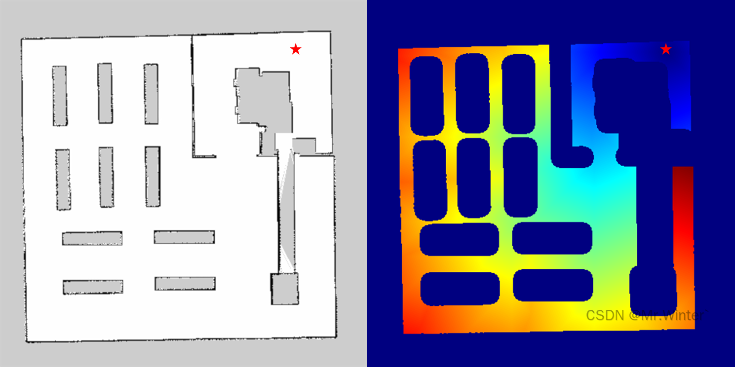
这是计算的代价势场可视化效果，红色五角星代表终点位置，约接近深蓝色代表与终点的最短距离越小，越接近红色则表示越远

3 算法仿真

ROS_C_102">3.1 ROS C++仿真

核心代码如下所示

bool GradientPathPlanner::plan(const Point3d& start, const Point3d& goal, Points3d& path, Points3d& expand)
{// clear vectorpath.clear();expand.clear();unsigned int sx = static_cast<unsigned int>(m_start_x);unsigned int sy = static_cast<unsigned int>(m_start_y);unsigned int gx = static_cast<unsigned int>(m_goal_x);unsigned int gy = static_cast<unsigned int>(m_goal_y);if (obstacle_hmap_(sy, sx) > 0){path.push_back(start);unsigned int curr_mx = sx;unsigned int curr_my = sy;while (!(curr_mx == gx && curr_my == gy)){unsigned int min_mx = curr_mx;unsigned int min_my = curr_my;float curr_cost = obstacle_hmap_(curr_my, curr_mx);for (const auto& motion : motions_){int new_mx = static_cast<int>(curr_mx) + motion.x();int new_my = static_cast<int>(curr_my) + motion.y();if (new_mx >= 0 && new_mx < nx_ && new_my >= 0 && new_my < ny_){float new_cost = obstacle_hmap_(new_my, new_mx);if (new_cost >= 0 && new_cost < curr_cost){curr_cost = new_cost;min_mx = new_mx;min_my = new_my;}}}curr_mx = min_mx;curr_my = min_my;double wx, wy;costmap_->mapToWorld(curr_mx, curr_my, wx, wy);path.emplace_back(wx, wy);}return true;}return false;
}

3.2 Python仿真

核心代码如下所示

def plan(self, start: Point3d, goal: Point3d) -> Tuple[List[Point3d], List[Dict]]:"""Gradient-based motion plan function.Parameters:start (Point3d): The starting point of the planning path.goal (Point3d): The goal point of the planning path.Returns:path (List[Point3d]): The planned path from start to goal.visual_info (List[Dict]): Information for visualization"""self.obs_hmap = self.calObstacleHeuristic(self.grid_map, goal)start_x, start_y = round(start.x()), round(start.y())if self.obs_hmap[start_y, start_x] > 0:path = [start]cost = self.obs_hmap[start_y, start_x]curr_x, curr_y = start_x, start_ywhile not (curr_x == round(goal.x()) and curr_y == round(goal.y())):min_x, min_y = None, Nonecurr_cost = self.obs_hmap[curr_y, curr_x]for dy, dx, _ in self.motions:new_x = curr_x + dxnew_y = curr_y + dyif 0 <= new_x < self.env.x_range and 0 <= new_y < self.env.y_range:new_cost = self.obs_hmap[new_y, new_x]if new_cost >= 0 and new_cost < curr_cost:curr_cost = new_costmin_x, min_y = new_x, new_ycurr_x = min_xcurr_y = min_ypath.append(Point3d(curr_x, curr_y))LOG.INFO(f"{str(self)} PathPlanner Planning Successfully. Cost: {cost}")return path

完整工程代码请联系下方博主名片获取

---

🔥 更多精彩专栏：

• 《ROS从入门到精通》
• 《Pytorch深度学习实战》
• 《机器学习强基计划》
• 《运动规划实战精讲》
• …

👇源码获取 · 技术交流 · 抱团学习 · 咨询分享 请联系👇