Multiple Variable Linear Regression
- 1、问题描述
- 1.1 包含样例的X矩阵
- 1.2 参数向量 w, b
- 2、多变量的模型预测
- 2.1 逐元素进行预测
- 2.2 向量点积进行预测
- 3、多变量线性回归模型计算损失
- 4、多变量线性回归模型梯度下降
- 4.1 计算梯度
- 4.2梯度下降
首先,导入所需的库
import copy, math
import numpy as np
import matplotlib.pyplot as plt
plt.style.use('./deeplearning.mplstyle')
np.set_printoptions(precision=2)  # reduced display precision on numpy arrays
1、问题描述
使用房价预测的示例来构建线性回归模型。训练数据集包含三个样本,每个样本有四个特征(面积、卧室数、楼层数和年龄),如下表所示。这里的面积以平方英尺(sqft)为单位。
| Size (sqft) | Number of Bedrooms | Number of floors | Age of Home | Price (1000s dollars) |
|---|---|---|---|---|
| 2104 | 5 | 1 | 45 | 460 |
| 1416 | 3 | 2 | 40 | 232 |
| 852 | 2 | 1 | 35 | 178 |
使用这些值构建线性回归模型,从而可以预测其他房屋的价格。例如,给定一个1200平方英尺、3个卧室、1层楼、40岁的房屋,可以用模型来预测其价格。
根据表格数据创建 X_train 和 y_train 变量。
X_train = np.array([[2104, 5, 1, 45], [1416, 3, 2, 40], [852, 2, 1, 35]])
y_train = np.array([460, 232, 178])
1.1 包含样例的X矩阵
与上面的表格类似,样例被存储在一个 NumPy 矩阵X_train 中。矩阵中的每一行表示一个样例。当有 m m m 个训练样例,每个样例有 n n n 个特征时, X \mathbf{X} X 是一个维度为 ( m m m, n n n) 的矩阵(m 行,n 列)。
X = ( x 0 ( 0 ) x 1 ( 0 ) ⋯ x n − 1 ( 0 ) x 0 ( 1 ) x 1 ( 1 ) ⋯ x n − 1 ( 1 ) ⋯ x 0 ( m − 1 ) x 1 ( m − 1 ) ⋯ x n − 1 ( m − 1 ) ) \mathbf{X} = \begin{pmatrix} x^{(0)}_0 & x^{(0)}_1 & \cdots & x^{(0)}_{n-1} \\ x^{(1)}_0 & x^{(1)}_1 & \cdots & x^{(1)}_{n-1} \\ \cdots \\ x^{(m-1)}_0 & x^{(m-1)}_1 & \cdots & x^{(m-1)}_{n-1} \end{pmatrix} X= x0(0)x0(1)⋯x0(m−1)x1(0)x1(1)x1(m−1)⋯⋯⋯xn−1(0)xn−1(1)xn−1(m−1)
notation:
- x ( i ) \mathbf{x}^{(i)} x(i) 是包含第 i 个样例的向量。 x ( i ) = ( x 0 ( i ) , x 1 ( i ) , ⋯ , x n − 1 ( i ) ) \mathbf{x}^{(i)}= (x^{(i)}_0, x^{(i)}_1, \cdots,x^{(i)}_{n-1}) x(i)=(x0(i),x1(i),⋯,xn−1(i))
- x j ( i ) x^{(i)}_j xj(i) 是第 i 个样例中的第 j 个元素。圆括号中的上标表示样例编号,而下标表示元素编号。
# data is stored in numpy array/matrix
print(f"X Shape: {X_train.shape}, X Type:{type(X_train)})")
print(X_train)
print(f"y Shape: {y_train.shape}, y Type:{type(y_train)})")
print(y_train)
1.2 参数向量 w, b
- w \mathbf{w} w 是具有 n n n 个元素的向量
- 每个元素包含一个特征相关的参数
- i在我们的数据集中, n = 4.
- 将这表示为列向量
w = ( w 0 w 1 ⋯ w n − 1 ) \mathbf{w} = \begin{pmatrix} w_0 \\ w_1 \\ \cdots\\ w_{n-1} \end{pmatrix} w= w0w1⋯wn−1
- b b b 是一个标量参数
为了演示, w \mathbf{w} w 和 b b b 将被加载为一些初始选定的值,这些值接近最优解。 w \mathbf{w} w 是一个一维的 NumPy 向量。
b_init = 785.1811367994083
w_init = np.array([ 0.39133535, 18.75376741, -53.36032453, -26.42131618])
print(f"w_init shape: {w_init.shape}, b_init type: {type(b_init)}")
2、多变量的模型预测
多变量的线性回归模型的预测可以表示为:
f w , b ( x ) = w 0 x 0 + w 1 x 1 + . . . + w n − 1 x n − 1 + b (1) f_{\mathbf{w},b}(\mathbf{x}) = w_0x_0 + w_1x_1 +... + w_{n-1}x_{n-1} + b \tag{1} fw,b(x)=w0x0+w1x1+...+wn−1xn−1+b(1)
或用向量表示:
f w , b ( x ) = w ⋅ x + b (2) f_{\mathbf{w},b}(\mathbf{x}) = \mathbf{w} \cdot \mathbf{x} + b \tag{2} fw,b(x)=w⋅x+b(2)
其中 ⋅ \cdot ⋅ 是向量点积
2.1 逐元素进行预测
之前的预测是将一个特征值乘以一个参数,然后再加上一个偏置参数。将之前的预测直接扩展到多个特征的实现,可以通过循环遍历每个元素,在每个元素上进行乘法操作,然后在最后加上偏置参数来实现。
def predict_single_loop(x, w, b): """single predict using linear regressionArgs:x (ndarray): Shape (n,) example with multiple featuresw (ndarray): Shape (n,) model parameters b (scalar): model parameter Returns:p (scalar): prediction"""n = x.shape[0]p = 0for i in range(n):p_i = x[i] * w[i] p = p + p_i p = p + b return p
# get a row from our training data
x_vec = X_train[0,:]
print(f"x_vec shape {x_vec.shape}, x_vec value: {x_vec}")# make a prediction
f_wb = predict_single_loop(x_vec, w_init, b_init)
print(f"f_wb shape {f_wb.shape}, prediction: {f_wb}")
x_vec. 是一个具有四个元素的 1-D NumPy 向量, f_wb 是一个标量。
2.2 向量点积进行预测
使用NumPy的 np.dot() 对向量进行点积操作,加快预测速度。
def predict(x, w, b): """single predict using linear regressionArgs:x (ndarray): Shape (n,) example with multiple featuresw (ndarray): Shape (n,) model parameters b (scalar): model parameter Returns:p (scalar): prediction"""p = np.dot(x, w) + b return p
# get a row from our training data
x_vec = X_train[0,:]
print(f"x_vec shape {x_vec.shape}, x_vec value: {x_vec}")# make a prediction
f_wb = predict(x_vec,w_init, b_init)
print(f"f_wb shape {f_wb.shape}, prediction: {f_wb}")
运行后可以看到,向量点积和元素循环的结果是相同的。
3、多变量线性回归模型计算损失
多变量线性回归的损失函数 J ( w , b ) J(\mathbf{w},b) J(w,b) 方程如下:
J ( w , b ) = 1 2 m ∑ i = 0 m − 1 ( f w , b ( x ( i ) ) − y ( i ) ) 2 (3) J(\mathbf{w},b) = \frac{1}{2m} \sum\limits_{i = 0}^{m-1} (f_{\mathbf{w},b}(\mathbf{x}^{(i)}) - y^{(i)})^2 \tag{3} J(w,b)=2m1i=0∑m−1(fw,b(x(i))−y(i))2(3)
其中:
f w , b ( x ( i ) ) = w ⋅ x ( i ) + b (4) f_{\mathbf{w},b}(\mathbf{x}^{(i)}) = \mathbf{w} \cdot \mathbf{x}^{(i)} + b \tag{4} fw,b(x(i))=w⋅x(i)+b(4)
w \mathbf{w} w 和 x ( i ) \mathbf{x}^{(i)} x(i) 是向量。
具体实现如下:
def compute_cost(X, y, w, b): """compute costArgs:X (ndarray (m,n)): Data, m examples with n featuresy (ndarray (m,)) : target valuesw (ndarray (n,)) : model parameters b (scalar) : model parameterReturns:cost (scalar): cost"""m = X.shape[0]cost = 0.0for i in range(m): f_wb_i = np.dot(X[i], w) + b #(n,)(n,) = scalar (see np.dot)cost = cost + (f_wb_i - y[i])**2 #scalarcost = cost / (2 * m) #scalar return cost
# Compute and display cost using our pre-chosen optimal parameters.
cost = compute_cost(X_train, y_train, w_init, b_init)
print(f'Cost at optimal w : {cost}')
4、多变量线性回归模型梯度下降
多变量线性回归的梯度下降方程如下:
repeat until convergence: { w j = w j − α ∂ J ( w , b ) ∂ w j for j = 0..n-1 b = b − α ∂ J ( w , b ) ∂ b } \begin{align*} \text{repeat}&\text{ until convergence:} \; \lbrace \newline\; & w_j = w_j - \alpha \frac{\partial J(\mathbf{w},b)}{\partial w_j} \tag{5} \; & \text{for j = 0..n-1}\newline &b\ \ = b - \alpha \frac{\partial J(\mathbf{w},b)}{\partial b} \newline \rbrace \end{align*} repeat} until convergence:{wj=wj−α∂wj∂J(w,b)b =b−α∂b∂J(w,b)for j = 0..n-1(5)
其中,n是特征的数量,参数 w j w_j wj, b b b, 同时更新
∂ J ( w , b ) ∂ w j = 1 m ∑ i = 0 m − 1 ( f w , b ( x ( i ) ) − y ( i ) ) x j ( i ) ∂ J ( w , b ) ∂ b = 1 m ∑ i = 0 m − 1 ( f w , b ( x ( i ) ) − y ( i ) ) \begin{align} \frac{\partial J(\mathbf{w},b)}{\partial w_j} &= \frac{1}{m} \sum\limits_{i = 0}^{m-1} (f_{\mathbf{w},b}(\mathbf{x}^{(i)}) - y^{(i)})x_{j}^{(i)} \tag{6} \\ \frac{\partial J(\mathbf{w},b)}{\partial b} &= \frac{1}{m} \sum\limits_{i = 0}^{m-1} (f_{\mathbf{w},b}(\mathbf{x}^{(i)}) - y^{(i)}) \tag{7} \end{align} ∂wj∂J(w,b)∂b∂J(w,b)=m1i=0∑m−1(fw,b(x(i))−y(i))xj(i)=m1i=0∑m−1(fw,b(x(i))−y(i))(6)(7)
-
m 是训练数据集样例的个数
-
f w , b ( x ( i ) ) f_{\mathbf{w},b}(\mathbf{x}^{(i)}) fw,b(x(i)) 是模型的预测值, y ( i ) y^{(i)} y(i) 是目标值。
4.1 计算梯度
下面是方程(6)和(7)的实现
- 外循环m个样例.
- 对每个样例计算并累加 ∂ J ( w , b ) ∂ b \frac{\partial J(\mathbf{w},b)}{\partial b} ∂b∂J(w,b)
- 内循环n个特征:
- 对于每个 w j w_j wj计算 ∂ J ( w , b ) ∂ w j \frac{\partial J(\mathbf{w},b)}{\partial w_j} ∂wj∂J(w,b)
def compute_gradient(X, y, w, b): """Computes the gradient for linear regression Args:X (ndarray (m,n)): Data, m examples with n featuresy (ndarray (m,)) : target valuesw (ndarray (n,)) : model parameters b (scalar) : model parameterReturns:dj_dw (ndarray (n,)): The gradient of the cost w.r.t. the parameters w. dj_db (scalar): The gradient of the cost w.r.t. the parameter b. """m,n = X.shape #(number of examples, number of features)dj_dw = np.zeros((n,))dj_db = 0.for i in range(m): err = (np.dot(X[i], w) + b) - y[i] for j in range(n): dj_dw[j] = dj_dw[j] + err * X[i, j] dj_db = dj_db + err dj_dw = dj_dw / m dj_db = dj_db / m return dj_db, dj_dw
#Compute and display gradient
tmp_dj_db, tmp_dj_dw = compute_gradient(X_train, y_train, w_init, b_init)
print(f'dj_db at initial w,b: {tmp_dj_db}')
print(f'dj_dw at initial w,b: \n {tmp_dj_dw}')
4.2梯度下降
下面是方程(5)的实现
def gradient_descent(X, y, w_in, b_in, cost_function, gradient_function, alpha, num_iters): """Performs batch gradient descent to learn theta. Updates theta by taking num_iters gradient steps with learning rate alphaArgs:X (ndarray (m,n)) : Data, m examples with n featuresy (ndarray (m,)) : target valuesw_in (ndarray (n,)) : initial model parameters b_in (scalar) : initial model parametercost_function : function to compute costgradient_function : function to compute the gradientalpha (float) : Learning ratenum_iters (int) : number of iterations to run gradient descentReturns:w (ndarray (n,)) : Updated values of parameters b (scalar) : Updated value of parameter """# An array to store cost J and w's at each iteration primarily for graphing laterJ_history = []w = copy.deepcopy(w_in) #avoid modifying global w within functionb = b_infor i in range(num_iters):# Calculate the gradient and update the parametersdj_db,dj_dw = gradient_function(X, y, w, b) ##None# Update Parameters using w, b, alpha and gradientw = w - alpha * dj_dw ##Noneb = b - alpha * dj_db ##None# Save cost J at each iterationif i<100000: # prevent resource exhaustion J_history.append( cost_function(X, y, w, b))# Print cost every at intervals 10 times or as many iterations if < 10if i% math.ceil(num_iters / 10) == 0:print(f"Iteration {i:4d}: Cost {J_history[-1]:8.2f} ")return w, b, J_history #return final w,b and J history for graphing
测试一下
# initialize parameters
initial_w = np.zeros_like(w_init)
initial_b = 0.
# some gradient descent settings
iterations = 1000
alpha = 5.0e-7
# run gradient descent
w_final, b_final, J_hist = gradient_descent(X_train, y_train, initial_w, initial_b, compute_cost, compute_gradient, alpha, iterations)
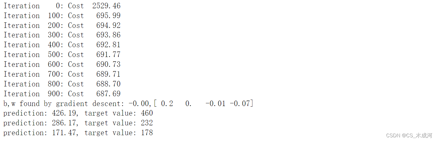
print(f"b,w found by gradient descent: {b_final:0.2f},{w_final} ")
m,_ = X_train.shape
for i in range(m):print(f"prediction: {np.dot(X_train[i], w_final) + b_final:0.2f}, target value: {y_train[i]}")
绘图可视化损失和迭代步数
# plot cost versus iteration
fig, (ax1, ax2) = plt.subplots(1, 2, constrained_layout=True, figsize=(12, 4))
ax1.plot(J_hist)
ax2.plot(100 + np.arange(len(J_hist[100:])), J_hist[100:])
ax1.set_title("Cost vs. iteration");  ax2.set_title("Cost vs. iteration (tail)")
ax1.set_ylabel('Cost')             ;  ax2.set_ylabel('Cost')
ax1.set_xlabel('iteration step')   ;  ax2.set_xlabel('iteration step')
plt.show()
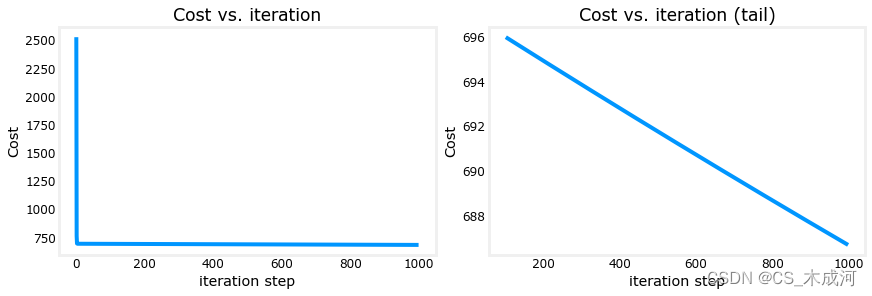
由此可以看出,损失仍在下降,而我们的预测并不是非常准确。下一个博客将探讨如何改进这一点。