文章目录

简单分类模型 - 逻辑回归
- 1.1 准备数据
- 1.2 定义假设函数
- - - Sigmoid 函数
- 1.3 定义代价函数
- 1.4 定义梯度下降算法
- - - gradient descent(梯度下降)
- 1.5 绘制决策边界
- 1.6 计算准确率
- 1.7 试试用Sklearn来解决
- 2.1 准备数据(试试第二个例子)
- 2.2 假设函数与前h相同
- 2.3 代价函数与前相同
- 2.4 梯度下降算法与前相同
- 2.5 欠拟合的了（模型过于简单，增加一些多项式特征）
- 2.6 定义正则化项的代价函数
- - - regularized cost（正则化代价函数）
- 2.7 定义正则化的梯度下降算法
- 实验1 计算基于正则化得到的准确率
- 2.8 试试sklearn
- 参考
- - 3.1 准备数据
- 实验2 完成3.2 调用逻辑回归模型完成分类
- - 3.2 调用普通的逻辑回归模型来进行多分类(调用1.4的梯度下降算法)
- 实验3 完成3.3 调用正则化的逻辑回归模型完成分类
- - 3.3调用正则化的逻辑回归模型来进行多分类(调用2.7的梯度下降算法)
- 实验4 完成3.3 调用SKLEARN完成分类
- - 3.4 调用SKLEARN

简单分类模型 - 逻辑回归

在这一次练习中，我们将要实现逻辑回归并且应用到一个分类任务。我们还将通过将正则化加入训练算法，来提高算法的鲁棒性，并用更复杂的情形来测试它。

1.1 准备数据

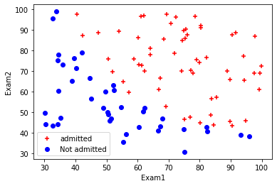
本实验的数据包含两个变量(评分1和评分2，可以看作是特征),某大学的管理者，想通过申请学生两次测试的评分，来决定他们是否被录取。因此，构建一个可以基于两次测试评分来评估录取可能性的分类模型。

import numpy as np
import pandas as pd
import matplotlib.pyplot as plt

#利用pandas显示数据
path = 'ex2data1.txt'
data = pd.read_csv(path, header=None, names=['Exam1', 'Exam2', 'Admitted'])
data.head()

	Exam1	Exam2	Admitted
0	34.623660	78.024693	0
1	30.286711	43.894998	0
2	35.847409	72.902198	0
3	60.182599	86.308552	1
4	79.032736	75.344376	1

data.info()

<class 'pandas.core.frame.DataFrame'>
RangeIndex: 100 entries, 0 to 99
Data columns (total 3 columns):#   Column    Non-Null Count  Dtype  
---  ------    --------------  -----  0   Exam1     100 non-null    float641   Exam2     100 non-null    float642   Admitted  100 non-null    int64  
dtypes: float64(2), int64(1)
memory usage: 2.5 KB

#看看数据的形状
data.shape

(100, 3)

让我们创建两个分数的散点图，并使用颜色编码来可视化，如果样本是正的（被接纳）或负的（未被接纳）。

positive_index=data["Admitted"].isin([1])
negative_index=data["Admitted"].isin([0])

positive_index

0     False
1     False
2     False
3      True
4      True...  
95     True
96     True
97     True
98     True
99     True
Name: Admitted, Length: 100, dtype: bool

plt.scatter(data[positive_index]["Exam1"],data[positive_index]["Exam2"],color="red",marker="+")
plt.scatter(data[negative_index]["Exam1"],data[negative_index]["Exam2"],color="blue",marker="o")
plt.legend(["admitted","Not admitted"])
plt.xlabel("Exam1")
plt.ylabel("Exam2")
plt.show()

positive = data[data['Admitted'].isin([1])]
negative = data[data['Admitted'].isin([0])]fig, ax = plt.subplots(figsize=(6,4))
ax.scatter(positive['Exam1'],positive['Exam2'],s=50,c='b',marker='o',label='Admitted')
ax.scatter(negative['Exam1'],negative['Exam2'],s=50,c='r',marker='x',label='Not Admitted')
ax.legend()
ax.set_xlabel('Exam 1 Score')
ax.set_ylabel('Exam 2 Score')
plt.show()

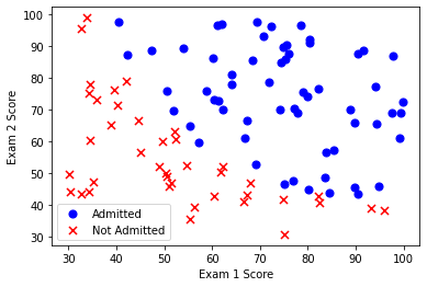
看起来在两类间，有一个清晰的决策边界。现在我们需要实现逻辑回归，那样就可以训练一个模型来预测结果。

#准备训练数据
col_num=data.shape[1]
X=data.iloc[:,:col_num-1]
y=data.iloc[:,col_num-1]

X.insert(0,"ones",1)
X.shape

(100, 3)

X=X.values
X.shape

(100, 3)

y=y.values
y.shape

(100,)

1.2 定义假设函数

Sigmoid 函数

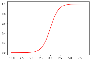
$g$ 代表一个常用的逻辑函数（logistic function）为 $S$ 形函数（Sigmoid function），公式为：
$g(z)=\frac{1}{1+{{e}^{-z}}}$
合起来，我们得到逻辑回归模型的假设函数：
${{h}}\left( x \right)=\frac{1}{1+{{e}^{-{{w }^{T}}x}}}$

def sigmoid(z):return 1 / (1 + np.exp(-z))

让我们做一个快速的检查，来确保它可以工作。

nums = np.arange(-10, 10, step=1)
fig, ax = plt.subplots(figsize=(6, 4))
ax.plot(nums, sigmoid(nums), 'r')
plt.show()

w=np.zeros((X.shape[1],1))

#定义假设函数h(x)=1/(1+exp^(-w.Tx))
def h(X,w):z=X@wh=sigmoid(z)return h

1.3 定义代价函数

y_hat=sigmoid(X@w)

X.shape,y.shape,np.log(y_hat).shape

((100, 3), (100,), (100, 1))

现在，我们需要编写代价函数来评估结果。
代价函数：
$J\left(w\right)=-\frac{1}{m}\sum\limits_{i=1}^{m}{({{y}^{(i)}}\log \left( {h}\left( {{x}^{(i)}} \right) \right)+\left( 1-{{y}^{(i)}} \right)\log \left( 1-{h}\left( {{x}^{(i)}} \right) \right))}$

#代价函数构造
def cost(X,w,y):#当X(m,n+1),y(m,),w(n+1,1)y_hat=sigmoid(X@w)right=np.multiply(y.ravel(),np.log(y_hat).ravel())+np.multiply((1-y).ravel(),np.log(1-y_hat).ravel())cost=-np.sum(right)/X.shape[0]return cost

#设置初始的权值
w=np.zeros((X.shape[1],1))
#查看初始的代价
cost(X,w,y)

0.6931471805599453

看起来不错，接下来，我们需要一个函数来计算我们的训练数据、标签和一些参数 $w$ 的梯度。

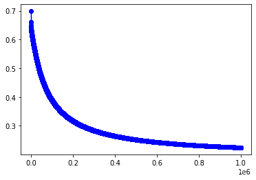
1.4 定义梯度下降算法

gradient descent(梯度下降)

这是批量梯度下降（batch gradient descent）
转化为向量化计算： $\frac{1}{m} X^T( Sigmoid(XW) - y )$
$\frac{\partial J\left( w \right)}{\partial {{w }_{j}}}=\frac{1}{m}\sum\limits_{i=1}^{m}{({{h}}\left( {{x}^{(i)}} \right)-{{y}^{(i)}})x_{_{j}}^{(i)}}$

def grandient(X,y,iter_num,alpha):y=y.reshape((X.shape[0],1))w=np.zeros((X.shape[1],1))cost_lst=[]for i in range(iter_num):y_pred=h(X,w)-ytemp=np.zeros((X.shape[1],1))for j in range(X.shape[1]):right=np.multiply(y_pred.ravel(),X[:,j])gradient=1/(X.shape[0])*(np.sum(right))temp[j,0]=w[j,0]-alpha*gradientw=tempcost_lst.append(cost(X,w,y.ravel()))return w,cost_lst

iter_num,alpha=1000000,0.001
w,cost_lst=grandient(X,y,iter_num,alpha)

cost_lst[iter_num-1]

0.22465416189188264

plt.plot(range(iter_num),cost_lst,"b-o")

[<matplotlib.lines.Line2D at 0x14224c08190>]

Xw—X(m,n) w (n,1)

array([[-15.39517866],[  0.12825989],[  0.12247929]])

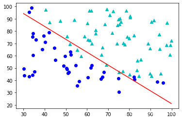
1.5 绘制决策边界

0=w[0,0]+w[1,0]*x1+w[2,0]*x2,令y=0 可以得到x2和x1的关系为
x2=(-w[0,0]-w[1,0]*x1)/w[2,0]

#绘图
x_exma1=np.linspace(data["Exam1"].min(),data["Exam1"].max(),100)
x2=(-w[0,0]-w[1,0]*x_exma1)/(w[2,0])
plt.plot(x_exma1,x2,"r-")
plt.scatter(data[positive_index]["Exam1"],data[positive_index]["Exam2"],color="c",marker="^")
plt.scatter(data[negative_index]["Exam1"],data[negative_index]["Exam2"],color="b",marker="o")
plt.show()

1.6 计算准确率

如何用我们所学的参数w来为数据集X输出预测，来给我们的分类器的训练精度打分。
逻辑回归模型的假设函数：
${{h}}\left( x \right)=\frac{1}{1+{{e}^{-{{w }^{T}}X}}}$

当 ${{h}}$ 大于等于0.5时，预测 y=1

当 ${{h}}$ 小于0.5时，预测 y=0 。

y_p_true=(h(X,w)>0.5).ravel()
y_p_true

array([False, False, False,  True,  True, False,  True, False,  True,True,  True, False,  True,  True, False,  True, False, False,True,  True, False,  True, False, False,  True,  True,  True,True, False, False,  True,  True, False, False, False, False,True,  True, False, False,  True, False,  True,  True, False,False,  True,  True,  True,  True,  True,  True,  True, False,False, False,  True,  True,  True,  True,  True, False, False,False, False, False,  True, False,  True,  True, False,  True,True,  True,  True,  True,  True,  True, False,  True,  True,True,  True, False,  True,  True, False,  True,  True, False,True,  True, False,  True,  True,  True,  True,  True, False,True])

y_p_pred=(data["Admitted"]==1).values
y_p_pred

array([False, False, False,  True,  True, False,  True,  True,  True,True, False, False,  True,  True, False,  True,  True, False,True,  True, False,  True, False, False,  True,  True,  True,False, False, False,  True,  True, False,  True, False, False,False,  True, False, False,  True, False,  True, False, False,False,  True,  True,  True,  True,  True,  True,  True, False,False, False,  True, False,  True,  True,  True, False, False,False, False, False,  True, False,  True,  True, False,  True,True,  True,  True,  True,  True,  True, False, False,  True,True,  True,  True,  True,  True, False,  True,  True, False,True,  True, False,  True,  True,  True,  True,  True,  True,True])

np.sum(y_p_pred==y_p_true)/X.shape[0]

0.89

1.7 试试用Sklearn来解决

from sklearn.linear_model import LogisticRegression
clf = LogisticRegression().fit(X, y)
clf.score(X,y)

0.89

clf.predict(X)

array([0, 0, 0, 1, 1, 0, 1, 0, 1, 1, 1, 0, 1, 1, 0, 1, 0, 0, 1, 1, 0, 1,0, 0, 1, 1, 1, 1, 0, 0, 1, 1, 0, 0, 0, 0, 1, 1, 0, 0, 1, 0, 1, 1,0, 0, 1, 1, 1, 1, 1, 1, 1, 0, 0, 0, 1, 1, 1, 1, 1, 0, 0, 0, 0, 0,1, 0, 1, 1, 0, 1, 1, 1, 1, 1, 1, 1, 0, 1, 1, 1, 1, 0, 1, 1, 0, 1,1, 0, 1, 1, 0, 1, 1, 1, 1, 1, 0, 1], dtype=int64)

np.array([1 if item>0.5 else 0 for item in h(X,w)])

array([0, 0, 0, 1, 1, 0, 1, 0, 1, 1, 1, 0, 1, 1, 0, 1, 0, 0, 1, 1, 0, 1,0, 0, 1, 1, 1, 1, 0, 0, 1, 1, 0, 0, 0, 0, 1, 1, 0, 0, 1, 0, 1, 1,0, 0, 1, 1, 1, 1, 1, 1, 1, 0, 0, 0, 1, 1, 1, 1, 1, 0, 0, 0, 0, 0,1, 0, 1, 1, 0, 1, 1, 1, 1, 1, 1, 1, 0, 1, 1, 1, 1, 0, 1, 1, 0, 1,1, 0, 1, 1, 0, 1, 1, 1, 1, 1, 0, 1])

np.argmax(clf.predict_proba(X),axis=1)

array([0, 0, 0, 1, 1, 0, 1, 0, 1, 1, 1, 0, 1, 1, 0, 1, 0, 0, 1, 1, 0, 1,0, 0, 1, 1, 1, 1, 0, 0, 1, 1, 0, 0, 0, 0, 1, 1, 0, 0, 1, 0, 1, 1,0, 0, 1, 1, 1, 1, 1, 1, 1, 0, 0, 0, 1, 1, 1, 1, 1, 0, 0, 0, 0, 0,1, 0, 1, 1, 0, 1, 1, 1, 1, 1, 1, 1, 0, 1, 1, 1, 1, 0, 1, 1, 0, 1,1, 0, 1, 1, 0, 1, 1, 1, 1, 1, 0, 1], dtype=int64)

X.shape,y.shape

((100, 3), (100,))

from sklearn.datasets import load_iris
from sklearn.linear_model import LogisticRegression
y
clf = LogisticRegression().fit(X, y)
clf.predict(X)

array([0, 0, 0, 1, 1, 0, 1, 0, 1, 1, 1, 0, 1, 1, 0, 1, 0, 0, 1, 1, 0, 1,0, 0, 1, 1, 1, 1, 0, 0, 1, 1, 0, 0, 0, 0, 1, 1, 0, 0, 1, 0, 1, 1,0, 0, 1, 1, 1, 1, 1, 1, 1, 0, 0, 0, 1, 1, 1, 1, 1, 0, 0, 0, 0, 0,1, 0, 1, 1, 0, 1, 1, 1, 1, 1, 1, 1, 0, 1, 1, 1, 1, 0, 1, 1, 0, 1,1, 0, 1, 1, 0, 1, 1, 1, 1, 1, 0, 1], dtype=int64)

clf.predict(X).shape

(100,)

y.shape

(100,)

np.sum(clf.predict(X)==y.ravel())/np.sum(X.shape[0])

0.89

#所以分类问题中的score用的是准确率
clf.score(X,y)

0.89

我们的逻辑回归分类器预测正确，如果一个学生被录取或没有录取，达到89%的精确度。不坏！记住，这是训练集的准确性。我们没有保持住了设置或使用交叉验证得到的真实逼近，所以这个数字有可能高于其真实值（这个话题将在以后说明）。

2.1 准备数据(试试第二个例子)

在训练的第二部分，我们将要通过加入正则项提升逻辑回归算。简而言之，正则化是成本函数中的一个术语，它使算法更倾向于“更简单”的模型（在这种情况下，模型将更小的系数）。这个理论助于减少过拟合，提高模型的泛化能力。

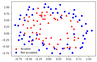
设想你是工厂的生产主管，你有一些芯片在两次测试中的测试结果。对于这两次测试，你想决定是否芯片要被接受或抛弃。为了帮助你做出艰难的决定，你拥有过去芯片的测试数据集，从其中你可以构建一个逻辑回归模型。

和第一部分很像，从数据可视化开始吧！

#读取文件'ex2data2.txt'的数据
path="ex2data2.txt"
data2=pd.read_csv(path,header=None,names=["Test1","Test2","Accepted"])
data2.head()

	Test1	Test2	Accepted
0	0.051267	0.69956	1
1	-0.092742	0.68494	1
2	-0.213710	0.69225	1
3	-0.375000	0.50219	1
4	-0.513250	0.46564	1

#可视化数据
positive_index=data2["Accepted"]==1
negative_index=data2["Accepted"]==0
plt.scatter(data2[positive_index]["Test1"],data2[positive_index]["Test2"],color="r",marker="^")
plt.scatter(data2[negative_index]["Test1"],data2[negative_index]["Test2"],color="b",marker="o")
plt.legend(["Accpted","Not accepted"])
plt.show()

X2=data2.iloc[:,:2]
y2=data2.iloc[:,2]
X2.insert(0,"ones",1)
X2.shape,y2.shape

((118, 3), (118,))

X2=X2.values
y2=y2.values

2.2 假设函数与前h相同

2.3 代价函数与前相同

2.4 梯度下降算法与前相同

iter_num,alpha=600000,0.0005
w,cost_lst=grandient(X2,y2,iter_num,alpha)

#绘制误差曲线
plt.plot(range(iter_num),cost_lst,"b-o")

[<matplotlib.lines.Line2D at 0x1422d45e970>]

#看看准确率有多少
y_pred=[1 if item>=0.5 else 0  for item in sigmoid(X2@w).ravel()]
y_pred=np.array(y_pred)
y_pred.shape

(118,)

y2.shape

(118,)

np.sum(y_pred==y2)

np.sum(y_pred==y2)/y2.shape[0]

0.5508474576271186

y_pred=[1 if item>=0.5 else 0  for item in sigmoid(X2@w).ravel()]
y_pred=np.array(y_pred)
np.sum(y_pred==y2)/y2.shape[0]

0.5508474576271186

2.5 欠拟合的了（模型过于简单，增加一些多项式特征）

path="ex2data2.txt"
data2=pd.read_csv(path,header=None,names=["Test1","Test2","Accepted"])
data2.head()

	Test1	Test2	Accepted
0	0.051267	0.69956	1
1	-0.092742	0.68494	1
2	-0.213710	0.69225	1
3	-0.375000	0.50219	1
4	-0.513250	0.46564	1

#为数据框增加多列多项式特征
def poly_feature(data2,degree):x1=data2["Test1"]x2=data2["Test2"]items=[]for i in range(degree+1):for j in range(degree-i+1):data2["F"+str(i)+str(j)]=np.power(x1,i)*np.power(x2,j)items.append("(x1**{})*(x2**{})".format(i,j))data2=data2.drop(["Test1","Test2"],axis=1)return data2,items
data2,items=poly_feature(data2,4)

data2.shape

(118, 16)

data2.head(5)

	Accepted	F00	F01	F02	F03	F04	F10	F11	F12	F13	F20	F21	F22	F30	F31	F40
0	1	1.0	0.69956	0.489384	0.342354	0.239497	0.051267	0.035864	0.025089	0.017551	0.002628	0.001839	0.001286	0.000135	0.000094	0.000007
1	1	1.0	0.68494	0.469143	0.321335	0.220095	-0.092742	-0.063523	-0.043509	-0.029801	0.008601	0.005891	0.004035	-0.000798	-0.000546	0.000074
2	1	1.0	0.69225	0.479210	0.331733	0.229642	-0.213710	-0.147941	-0.102412	-0.070895	0.045672	0.031616	0.021886	-0.009761	-0.006757	0.002086
3	1	1.0	0.50219	0.252195	0.126650	0.063602	-0.375000	-0.188321	-0.094573	-0.047494	0.140625	0.070620	0.035465	-0.052734	-0.026483	0.019775
4	1	1.0	0.46564	0.216821	0.100960	0.047011	-0.513250	-0.238990	-0.111283	-0.051818	0.263426	0.122661	0.057116	-0.135203	-0.062956	0.069393

X2=data2.iloc[:,1:data2.shape[1]-1]
y2=data2.iloc[:,0]
X2.shape,y.shape

((118, 14), (100,))

X2

	F00	F01	F02	F03	F04	F10	F11	F12	F13	F20	F21	F22	F30	F31
0	1.0	0.699560	0.489384	0.342354	2.394969e-01	0.051267	0.035864	0.025089	0.017551	0.002628	0.001839	0.001286	1.347453e-04	9.426244e-05
1	1.0	0.684940	0.469143	0.321335	2.200950e-01	-0.092742	-0.063523	-0.043509	-0.029801	0.008601	0.005891	0.004035	-7.976812e-04	-5.463638e-04
2	1.0	0.692250	0.479210	0.331733	2.296423e-01	-0.213710	-0.147941	-0.102412	-0.070895	0.045672	0.031616	0.021886	-9.760555e-03	-6.756745e-03
3	1.0	0.502190	0.252195	0.126650	6.360222e-02	-0.375000	-0.188321	-0.094573	-0.047494	0.140625	0.070620	0.035465	-5.273438e-02	-2.648268e-02
4	1.0	0.465640	0.216821	0.100960	4.701118e-02	-0.513250	-0.238990	-0.111283	-0.051818	0.263426	0.122661	0.057116	-1.352032e-01	-6.295600e-02
...	...	...	...	...	...	...	...	...	...	...	...	...	...	...
113	1.0	0.538740	0.290241	0.156364	8.423971e-02	-0.720620	-0.388227	-0.209153	-0.112679	0.519293	0.279764	0.150720	-3.742131e-01	-2.016035e-01
114	1.0	0.494880	0.244906	0.121199	5.997905e-02	-0.593890	-0.293904	-0.145447	-0.071979	0.352705	0.174547	0.086380	-2.094682e-01	-1.036616e-01
115	1.0	0.999270	0.998541	0.997812	9.970832e-01	-0.484450	-0.484096	-0.483743	-0.483390	0.234692	0.234520	0.234349	-1.136964e-01	-1.136134e-01
116	1.0	0.999270	0.998541	0.997812	9.970832e-01	-0.006336	-0.006332	-0.006327	-0.006323	0.000040	0.000040	0.000040	-2.544062e-07	-2.542205e-07
117	1.0	-0.030612	0.000937	-0.000029	8.781462e-07	0.632650	-0.019367	0.000593	-0.000018	0.400246	-0.012252	0.000375	2.532156e-01	-7.751437e-03

118 rows × 14 columns

y2

0      1
1      1
2      1
3      1
4      1..
113    0
114    0
115    0
116    0
117    0
Name: Accepted, Length: 118, dtype: int64

X2=X2.values
y2=y2.values

X2.shape,y2.shape

((118, 14), (118,))

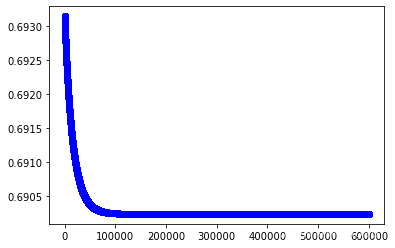
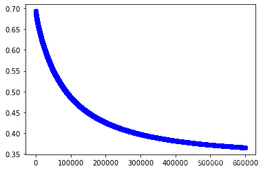
#虽然加了多项式特征，但是其他地方不需要改变
iter_num,alpha=600000,0.001
w,cost_lst=grandient(X2,y2,iter_num,alpha)
w,cost_lst

(array([[ 3.03503577],[ 3.20158942],[-4.0495866 ],[-1.04983379],[-3.95636068],[ 2.0490215 ],[-3.40302089],[-0.79821365],[-1.23393575],[-7.32541507],[-1.41115593],[-1.80717912],[-0.54355034],[ 0.11775491]]),[0.6931399371004173,0.6931326952275558,0.6931254549404754,0.6931182162382921,0.693110979120122,0.6931037435850823,0.69309650963229,0.6930892772608634,0.6930820464699207,0.6930748172585808,0.6930675896259637,0.6930603635711893,0.6930531390933783,0.693045916191652,0.6930386948651323,0.6930314751129414,0.6930242569342021,0.6930170403280382,0.6930098252935735,0.6930026118299326,0.6929953999362406,0.6929881896116231,0.6929809808552065,0.6929737736661173,0.6929665680434831,0.6929593639864312,0.6929521614940908,0.6929449605655903,0.6929377612000593,0.6929305633966278,0.6929233671544265,0.6929161724725863,0.6929089793502394,0.6929017877865175,0.6928945977805535,0.6928874093314809,0.6928802224384333,0.6928730371005455,0.6928658533169517,0.6928586710867882,0.6928514904091909,0.6928443112832959,0.6928371337082408,0.6928299576831629,0.6928227832072007,0.6928156102794925,0.692808438899178,0.6928012690653973,0.6927941007772903,0.6927869340339977,0.6927797688346614,0.6927726051784232,0.6927654430644256,0.6927582824918116,0.6927511234597252,0.6927439659673101,0.6927368100137112,0.6927296555980735,0.6927225027195429,0.6927153513772657,0.6927082015703889,0.6927010532980594,0.6926939065594254,0.6926867613536353,0.6926796176798382,0.6926724755371833,0.6926653349248207,0.692658195841901,0.6926510582875753,0.6926439222609956,0.6926367877613135,0.6926296547876825,0.6926225233392544,0.6926153934151844,0.6926082650146258,0.6926011381367343,0.6925940127806647,0.6925868889455729,0.6925797666306154,0.6925726458349493,0.692565526557732,0.6925584087981212,0.6925512925552758,0.6925441778283548,0.6925370646165178,0.6925299529189249,0.6925228427347367,0.6925157340631142,0.6925086269032195,0.6925015212542147,0.6924944171152624,0.6924873144855257,0.692480213364169,0.6924731137503559,0.692466015643252,0.6924589190420221,0.6924518239458325,0.6924447303538497,0.6924376382652399,0.6924305476791713,0.6924234585948119,0.6924163710113299,0.6924092849278943,0.6924022003436747,0.6923951172578418,0.6923880356695654,0.692380955578017,0.6923738769823684,0.6923667998817915,0.6923597242754587,0.6923526501625441,0.6923455775422206,0.6923385064136628,0.6923314367760456,0.6923243686285434,0.6923173019703337,0.6923102368005914,0.6923031731184935,0.6922961109232177,0.6922890502139424,0.6922819909898448,0.6922749332501046,0.692267876993901,0.6922608222204141,0.692253768928824,0.6922467171183119,0.6922396667880594,0.6922326179372482,0.692225570565061,0.6922185246706808,0.6922114802532913,0.6922044373120759,0.69219739584622,0.692190355854908,0.692183317337326,0.6921762802926597,0.6921692447200962,0.6921622106188222,0.6921551779880252,0.6921481468268937,0.6921411171346162,0.6921340889103819,0.6921270621533807,0.6921200368628022,0.6921130130378376,0.6921059906776778,0.6920989697815146,0.6920919503485404,0.6920849323779475,0.6920779158689296,0.6920709008206801,0.6920638872323933,0.6920568751032641,0.6920498644324875,0.6920428552192593,0.692035847462776,0.6920288411622341,0.6920218363168312,0.6920148329257646,0.6920078309882332,0.692000830503435,0.6919938314705699,0.6919868338888373,0.6919798377574379,0.6919728430755722,0.6919658498424414,0.6919588580572479,0.6919518677191929,0.6919448788274806,0.6919378913813131,0.6919309053798947,0.6919239208224298,0.691916937708123,0.6919099560361796,0.6919029758058055,0.691895997016207,0.6918890196665908,0.6918820437561641,0.6918750692841349,0.6918680962497116,0.6918611246521027,0.6918541544905173,0.691847185764166,0.6918402184722583,0.6918332526140052,0.6918262881886181,0.6918193251953085,0.691812363633289,0.691805403501772,0.691798444799971,0.6917914875270996,0.6917845316823721,0.6917775772650034,0.6917706242742084,0.6917636727092031,0.6917567225692034,0.6917497738534262,0.6917428265610885,0.6917358806914085,0.691728936243604,0.6917219932168934,0.6917150516104965,0.6917081114236324,0.6917011726555214,0.6916942353053842,0.691687299372442,0.6916803648559162,0.691673431755029,0.6916665000690029,0.691659569797061,0.6916526409384272,0.691645713492325,0.6916387874579791,0.6916318628346149,0.6916249396214572,0.6916180178177327,0.6916110974226677,0.6916041784354889,0.6915972608554238,0.6915903446817003,0.6915834299135475,0.6915765165501937,0.691569604590868,0.6915626940348011,0.6915557848812225,0.6915488771293637,0.6915419707784556,0.6915350658277303,0.69152816227642,0.691521260123757,0.6915143593689757,0.6915074600113087,0.6915005620499908,0.6914936654842565,0.6914867703133412,0.6914798765364804,0.6914729841529099,0.691466093161867,0.6914592035625885,0.6914523153543117,0.6914454285362747,0.6914385431077166,0.6914316590678757,0.6914247764159921,0.6914178951513054,0.6914110152730563,0.6914041367804855,0.6913972596728342,0.6913903839493448,0.6913835096092594,0.6913766366518207,0.6913697650762726,0.6913628948818578,0.6913560260678212,0.6913491586334077,0.6913422925778623,0.6913354279004306,0.6913285646003587,0.6913217026768933,0.6913148421292818,0.6913079829567716,0.6913011251586102,0.691294268734047,0.6912874136823305,0.6912805600027101,0.6912737076944359,0.6912668567567581,0.6912600071889275,0.691253158990196,0.6912463121598151,0.691239466697037,0.6912326226011144,0.6912257798713006,0.6912189385068493,0.6912120985070148,0.6912052598710514,0.6911984225982147,0.6911915866877595,0.6911847521389427,0.69117791895102,0.6911710871232487,0.6911642566548867,0.6911574275451913,0.6911505997934211,0.6911437733988343,0.6911369483606911,0.6911301246782512,0.6911233023507742,0.6911164813775215,0.6911096617577531,0.691102843490732,0.6910960265757193,0.6910892110119781,0.6910823967987713,0.6910755839353621,0.6910687724210147,0.6910619622549933,0.6910551534365628,0.6910483459649887,0.6910415398395364,0.6910347350594729,0.6910279316240643,0.6910211295325772,0.6910143287842805,0.6910075293784415,0.6910007313143287,0.6909939345912114,0.6909871392083592,0.6909803451650415,0.6909735524605287,0.6909667610940924,0.6909599710650032,0.6909531823725328,0.6909463950159536,0.6909396089945385,0.6909328243075601,0.6909260409542926,0.6909192589340094,0.6909124782459855,0.6909056988894955,0.690898920863815,0.6908921441682196,0.6908853688019859,0.6908785947643907,0.6908718220547111,0.6908650506722244,0.6908582806162092,0.6908515118859441,0.6908447444807079,0.6908379783997801,0.6908312136424405,0.6908244502079699,0.6908176880956487,0.6908109273047588,0.6908041678345811,0.6907974096843985,0.6907906528534933,0.6907838973411485,0.690777143146648,0.6907703902692756,0.6907636387083155,0.6907568884630527,0.690750139532773,0.690743391916762,0.6907366456143056,0.6907299006246905,0.6907231569472044,0.6907164145811341,0.6907096735257682,0.690702933780395,0.6906961953443035,0.6906894582167828,0.690682722397123,0.6906759878846143,0.6906692546785472,0.6906625227782132,0.6906557921829036,0.6906490628919102,0.6906423349045264,0.6906356082200443,0.6906288828377575,0.6906221587569599,0.6906154359769455,0.6906087144970098,0.6906019943164466,0.6905952754345525,0.6905885578506235,0.6905818415639554,0.6905751265738461,0.690568412879592,0.6905617004804914,0.6905549893758427,0.6905482795649438,0.6905415710470946,0.6905348638215943,0.6905281578877431,0.6905214532448414,0.6905147498921895,0.6905080478290895,0.690501347054843,0.6904946475687516,0.6904879493701188,0.6904812524582472,0.6904745568324402,0.6904678624920019,0.6904611694362365,0.6904544776644493,0.6904477871759448,0.6904410979700292,0.6904344100460088,0.6904277234031898,0.6904210380408787,0.6904143539583844,0.6904076711550134,0.6904009896300746,0.6903943093828763,0.6903876304127281,0.6903809527189395,0.6903742763008206,0.6903676011576815,0.6903609272888331,0.6903542546935871,0.6903475833712557,0.69034091332115,0.6903342445425832,0.6903275770348686,0.6903209107973187,0.6903142458292487,0.6903075821299722,0.6903009196988041,0.6902942585350598,0.6902875986380544,0.6902809400071047,0.6902742826415266,0.6902676265406373,0.6902609717037543,0.6902543181301951,0.6902476658192781,0.6902410147703216,0.6902343649826451,0.6902277164555679,0.6902210691884098,0.6902144231804913,0.6902077784311333,0.690201134939657,0.6901944927053835,0.6901878517276353,0.6901812120057349,0.6901745735390051,0.6901679363267692,0.6901613003683511,0.6901546656630752,0.6901480322102651,0.6901414000092467,0.6901347690593452,0.6901281393598866,0.690121510910197,0.6901148837096033,0.6901082577574326,0.6901016330530122,0.6900950095956704,0.6900883873847353,0.6900817664195361,0.6900751466994021,0.6900685282236624,0.6900619109916476,0.6900552950026879,0.6900486802561143,0.6900420667512582,0.6900354544874515,0.6900288434640263,0.690022233680315,0.6900156251356507,0.6900090178293673,0.6900024117607981,0.6899958069292774,0.6899892033341402,0.6899826009747214,0.6899759998503566,0.6899693999603816,0.6899628013041332,0.6899562038809481,0.6899496076901628,0.6899430127311155,0.6899364190031444,0.6899298265055872,0.6899232352377836,0.6899166451990724,0.6899100563887932,0.6899034688062867,0.6898968824508926,0.6898902973219526,0.6898837134188075,0.6898771307407991,0.6898705492872698,0.6898639690575618,0.6898573900510188,0.6898508122669835,0.6898442357048,0.6898376603638127,0.689831086243366,0.6898245133428047,0.6898179416614751,0.689811371198722,0.6898048019538924,0.689798233926333,0.6897916671153906,0.6897851015204128,0.6897785371407474,0.6897719739757432,0.6897654120247485,0.6897588512871126,0.6897522917621844,0.6897457334493153,0.6897391763478544,0.689732620457153,0.6897260657765623,0.6897195123054336,0.6897129600431194,0.6897064089889716,0.6896998591423432,0.6896933105025878,0.6896867630690583,0.6896802168411088,0.6896736718180946,0.6896671279993697,0.6896605853842896,0.6896540439722101,0.6896475037624867,0.6896409647544766,0.6896344269475361,0.6896278903410226,0.689621354934294,0.6896148207267083,0.6896082877176235,0.6896017559063989,0.6895952252923941,0.689588695874968,0.6895821676534813,0.6895756406272939,0.6895691147957672,0.6895625901582623,0.6895560667141409,0.6895495444627653,0.6895430234034974,0.6895365035357004,0.6895299848587378,0.6895234673719729,0.6895169510747703,0.6895104359664939,0.6895039220465085,0.6894974093141799,0.6894908977688735,0.6894843874099555,0.6894778782367924,0.6894713702487508,0.6894648634451982,0.6894583578255021,0.6894518533890304,0.6894453501351522,0.6894388480632355,0.6894323471726499,0.6894258474627657,0.6894193489329519,0.6894128515825795,0.6894063554110188,0.6893998604176417,0.6893933666018192,0.6893868739629238,0.6893803825003278,0.6893738922134036,0.6893674031015249,0.689360915164065,0.6893544284003981,0.6893479428098981,0.6893414583919399,0.6893349751458988,0.6893284930711506,0.6893220121670708,0.6893155324330359,0.6893090538684223,0.6893025764726077,0.6892961002449691,0.6892896251848848,0.6892831512917327,0.6892766785648914,0.68927020700374,0.6892637366076584,0.6892572673760258,0.689250799308223,0.6892443324036301,0.6892378666616283,0.689231402081599,0.6892249386629243,0.6892184764049858,0.6892120153071661,0.6892055553688485,0.689199096589416,0.6891926389682527,0.689186182504742,0.6891797271982693,0.6891732730482184,0.6891668200539756,0.6891603682149255,0.6891539175304552,0.6891474679999502,0.6891410196227977,0.6891345723983848,0.6891281263260991,0.6891216814053285,0.6891152376354615,0.6891087950158865,0.6891023535459927,0.6890959132251698,0.6890894740528071,0.6890830360282953,0.689076599151025,0.6890701634203871,0.6890637288357729,0.6890572953965745,0.6890508631021836,0.6890444319519929,0.6890380019453953,0.6890315730817844,0.6890251453605535,0.6890187187810966,0.689012293342808,0.6890058690450832,0.688999445887317,0.6889930238689047,0.6889866029892425,0.6889801832477265,0.6889737646437539,0.6889673471767213,0.6889609308460263,0.6889545156510667,0.6889481015912406,0.688941688665947,0.6889352768745843,0.6889288662165526,0.6889224566912505,0.6889160482980794,0.6889096410364388,0.6889032349057299,0.6888968299053541,0.6888904260347121,0.688884023293207,0.6888776216802407,0.6888712211952157,0.6888648218375353,0.688858423606603,0.6888520265018226,0.6888456305225984,0.6888392356683349,0.6888328419384366,0.6888264493323096,0.6888200578493595,0.6888136674889918,0.6888072782506132,0.6888008901336309,0.6887945031374517,0.6887881172614835,0.6887817325051336,0.6887753488678109,0.6887689663489238,0.6887625849478818,0.6887562046640934,0.6887498254969691,0.6887434474459192,0.6887370705103535,0.6887306946896832,0.6887243199833197,0.6887179463906749,0.6887115739111601,0.6887052025441883,0.688698832289172,0.6886924631455241,0.6886860951126584,0.6886797281899885,0.6886733623769289,0.6886669976728934,0.688660634077298,0.6886542715895576,0.6886479102090873,0.6886415499353039,0.6886351907676235,0.6886288327054628,0.688622475748239,0.6886161198953701,0.6886097651462728,0.6886034115003662,0.6885970589570687,0.6885907075157992,0.6885843571759768,0.688578007937022,0.688571659798354,0.6885653127593935,0.6885589668195611,0.688552621978278,0.6885462782349664,0.6885399355890471,0.6885335940399426,0.688527253587076,0.6885209142298696,0.6885145759677471,0.6885082388001322,0.6885019027264487,0.688495567746121,0.6884892338585739,0.6884829010632325,0.6884765693595224,0.6884702387468692,0.6884639092246994,0.688457580792439,0.6884512534495155,0.688444927195356,0.6884386020293876,0.688432277951039,0.6884259549597384,0.6884196330549139,0.6884133122359953,0.6884069925024113,0.6884006738535923,0.6883943562889684,0.6883880398079698,0.6883817244100272,0.6883754100945724,0.6883690968610363,0.6883627847088507,0.6883564736374485,0.6883501636462622,0.6883438547347244,0.6883375469022686,0.6883312401483285,0.6883249344723381,0.6883186298737317,0.6883123263519442,0.6883060239064109,0.6882997225365669,0.688293422241848,0.6882871230216905,0.688280824875531,0.688274527802806,0.6882682318029532,0.6882619368754096,0.6882556430196136,0.6882493502350031,0.6882430585210174,0.6882367678770945,0.6882304783026743,0.6882241897971964,0.6882179023601008,0.688211615990828,0.6882053306888185,0.6881990464535135,0.6881927632843541,0.6881864811807826,0.688180200142241,0.6881739201681716,0.6881676412580173,0.688161363411221,0.6881550866272266,0.688148810905478,0.6881425362454192,0.6881362626464946,0.6881299901081493,0.6881237186298288,0.6881174482109782,0.688111178851044,0.6881049105494719,0.6880986433057091,0.6880923771192019,0.6880861119893985,0.6880798479157462,0.6880735848976928,0.6880673229346868,0.6880610620261772,0.6880548021716124,0.6880485433704425,0.6880422856221169,0.688036028926086,0.6880297732817994,0.688023518688709,0.6880172651462653,0.6880110126539196,0.6880047612111242,0.6879985108173311,0.6879922614719927,0.6879860131745617,0.6879797659244915,0.6879735197212354,0.6879672745642478,0.6879610304529822,0.6879547873868935,0.6879485453654369,0.6879423043880668,0.6879360644542397,0.6879298255634108,0.6879235877150365,0.687917350908574,0.6879111151434792,0.68790488041921,0.6878986467352243,0.6878924140909791,0.6878861824859337,0.6878799519195458,0.6878737223912752,0.6878674939005806,0.687861266446922,0.687855040029759,0.6878488146485524,0.6878425903027628,0.6878363669918508,0.6878301447152777,0.6878239234725055,0.6878177032629961,0.6878114840862118,0.6878052659416156,0.6877990488286697,0.6877928327468382,0.6877866176955842,0.6877804036743725,0.6877741906826668,0.6877679787199319,0.6877617677856327,0.6877555578792349,0.6877493490002041,0.687743141148006,0.6877369343221074,0.6877307285219747,0.687724523747075,0.6877183199968756,0.6877121172708444,0.6877059155684492,0.6876997148891582,0.6876935152324404,0.6876873165977645,0.6876811189846005,0.6876749223924173,0.6876687268206851,0.6876625322688749,0.6876563387364565,0.6876501462229011,0.6876439547276804,0.6876377642502658,0.6876315747901297,0.6876253863467437,0.6876191989195807,0.6876130125081141,0.6876068271118165,0.6876006427301624,0.6875944593626252,0.6875882770086794,0.6875820956677994,0.6875759153394605,0.6875697360231376,0.6875635577183067,0.6875573804244435,0.6875512041410243,0.6875450288675257,0.6875388546034246,0.6875326813481982,0.6875265091013244,0.6875203378622806,0.6875141676305453,0.6875079984055974,0.6875018301869149,0.6874956629739777,0.6874894967662654,0.687483331563257,0.6874771673644338,0.6874710041692756,0.6874648419772635,0.6874586807878786,0.6874525206006021,0.6874463614149161,0.6874402032303029,0.6874340460462444,0.6874278898622237,0.6874217346777238,0.6874155804922284,0.6874094273052211,0.6874032751161857,0.687397123924607,0.6873909737299688,0.6873848245317573,0.6873786763294574,0.6873725291225545,0.6873663829105352,0.6873602376928849,0.687354093469091,0.6873479502386403,0.6873418080010198,0.6873356667557176,0.6873295265022208,0.6873233872400182,0.6873172489685984,0.6873111116874501,0.6873049753960627,0.6872988400939255,0.6872927057805283,0.6872865724553615,0.6872804401179151,0.68727430876768,0.6872681784041478,0.6872620490268097,0.687255920635157,0.6872497932286825,0.6872436668068779,0.6872375413692363,0.68723141691525,0.6872252934444134,0.6872191709562195,0.6872130494501623,0.6872069289257362,0.6872008093824358,0.6871946908197555,0.6871885732371911,0.6871824566342382,0.6871763410103922,0.6871702263651496,0.6871641126980065,0.6871580000084602,0.6871518882960073,0.6871457775601456,0.6871396678003725,0.6871335590161864,0.6871274512070853,0.6871213443725684,0.6871152385121341,0.6871091336252817,0.6871030297115114,0.6870969267703225,0.6870908248012159,0.6870847238036913,0.68707862377725,0.6870725247213932,0.6870664266356225,0.6870603295194394,0.6870542333723462,0.6870481381938451,0.6870420439834392,0.6870359507406308,0.687029858464924,0.6870237671558223,0.6870176768128294,0.6870115874354497,0.6870054990231881,0.6869994115755486,0.6869933250920375,0.6869872395721597,0.6869811550154208,0.6869750714213273,0.6869689887893855,0.6869629071191022,0.6869568264099849,0.6869507466615399,0.6869446678732757,0.6869385900446999,0.6869325131753212,0.6869264372646477,0.6869203623121884,0.6869142883174523,0.6869082152799498,0.6869021431991895,0.6868960720746824,0.6868900019059384,0.6868839326924686,0.6868778644337838,0.6868717971293953,0.686865730778815,0.6868596653815545,0.6868536009371263,0.6868475374450429,0.6868414749048171,0.6868354133159618,0.6868293526779911,0.6868232929904182,0.6868172342527574,0.6868111764645234,0.68680511962523,0.6867990637343928,0.6867930087915272,0.6867869547961485,0.6867809017477724,0.6867748496459155,0.686768798490094,0.6867627482798252,0.6867566990146253,0.6867506506940125,0.6867446033175041,0.686738556884618,0.6867325113948729,0.686726466847787,0.6867204232428794,0.6867143805796693,0.6867083388576762,0.6867022980764199,0.6866962582354202,0.6866902193341977,0.6866841813722733,0.6866781443491677,0.6866721082644022,0.6866660731174986,0.6866600389079782,0.686654005635364,0.6866479732991783,0.6866419418989436,0.6866359114341828,0.6866298819044195,0.6866238533091775,0.686617825647981,0.6866117989203535,0.6866057731258198,0.6865997482639055,0.686593724334135,0.6865877013360339,0.686581679269128,0.6865756581329433,0.686569637927006,...])

w.shape

(14, 1)

cost_lst[iter_num-1]

0.365635134439536

#绘制误差曲线
plt.plot(range(iter_num),cost_lst,"b-o")

[<matplotlib.lines.Line2D at 0x1422d44cdc0>]

这时要重新绘图了
items

X2

array([[ 1.00000000e+00,  6.99560000e-01,  4.89384194e-01, ...,1.28625106e-03,  1.34745327e-04,  9.42624411e-05],[ 1.00000000e+00,  6.84940000e-01,  4.69142804e-01, ...,4.03513411e-03, -7.97681228e-04, -5.46363780e-04],[ 1.00000000e+00,  6.92250000e-01,  4.79210063e-01, ...,2.18864648e-02, -9.76055545e-03, -6.75674451e-03],...,[ 1.00000000e+00,  9.99270000e-01,  9.98540533e-01, ...,2.34349278e-01, -1.13696444e-01, -1.13613445e-01],[ 1.00000000e+00,  9.99270000e-01,  9.98540533e-01, ...,4.00913674e-05, -2.54406238e-07, -2.54220521e-07],[ 1.00000000e+00, -3.06120000e-02,  9.37094544e-04, ...,3.75068364e-04,  2.53215646e-01, -7.75143736e-03]])

X2.shape,w.shape

((118, 14), (14, 1))

y_pred=[1 if item>=0.5 else 0  for item in sigmoid(X2@w).ravel()]
y_pred=np.array(y_pred)
np.sum(y_pred==y2)/y2.shape[0]

0.8305084745762712

2.6 定义正则化项的代价函数

regularized cost（正则化代价函数）

$J\left( w \right)=\frac{1}{m}\sum\limits_{i=1}^{m}{[-{{y}^{(i)}}\log \left( {{h}}\left( {{x}^{(i)}} \right) \right)-\left( 1-{{y}^{(i)}} \right)\log \left( 1-{{h}}\left( {{x}^{(i)}} \right) \right)]}+\frac{\lambda }{2m}\sum\limits_{j=1}^{n}{w _{j}^{2}}$

w[:,0]

array([ 3.03503577,  3.20158942, -4.0495866 , -1.04983379, -3.95636068,2.0490215 , -3.40302089, -0.79821365, -1.23393575, -7.32541507,-1.41115593, -1.80717912, -0.54355034,  0.11775491])

#代价函数构造
def cost_reg(X,w,y,lambd):#当X(m,n+1),y(m,),w(n+1,1)y_hat=sigmoid(X@w)right1=np.multiply(y.ravel(),np.log(y_hat).ravel())+np.multiply((1-y).ravel(),np.log(1-y_hat).ravel())right2=(lambd/(2*X.shape[0]))*np.sum(np.power(w[1:,0],2))cost=-np.sum(right1)/X.shape[0]+right2return cost

cost(X2,w,y2)

0.365635134439536

lambd=2
cost_reg(X2,w,y2,lambd)

1.3874260376493517

2.7 定义正则化的梯度下降算法

如果我们要使用梯度下降法令这个代价函数最小化，因为我们未对 ${{w }_{0}}$ 进行正则化，所以梯度下降算法将分两种情形：

$KaTeX parse error: No such environment: align at position 7: \begin{̲a̲l̲i̲g̲n̲}̲ & 重复\text{ }…$

对上面的算法中 j=1,2,…,n 时的更新式子进行调整可得：
$}_{j}}:={{w }_{j}}(1-a\frac{\lambda }{m})-a\frac{1}{m}\sum\limits_{i=1}^{m}{({{h}_{w }}\left( {{x}^{(i)}} \right)-{{y}^{(i)}})x_{j}^{(i)}}$

def grandient_reg(X,w,y,iter_num,alpha,lambd):y=y.reshape((X.shape[0],1))w=np.zeros((X.shape[1],1))cost_lst=[] for i in range(iter_num):y_pred=h(X,w)-ytemp=np.zeros((X.shape[1],1))for j in range(0,X.shape[1]):if j==0:right_0=np.multiply(y_pred.ravel(),X[:,0])gradient_0=1/(X.shape[0])*(np.sum(right_0))temp[j,0]=w[j,0]-alpha*(gradient_0)else:right=np.multiply(y_pred.ravel(),X[:,j])reg=(lambd/X.shape[0])*w[j,0]gradient=1/(X.shape[0])*(np.sum(right))temp[j,0]=w[j,0]-alpha*(gradient+reg)          w=tempcost_lst.append(cost_reg(X,w,y,lambd))return w,cost_lst

iter_num,alpha,lambd=600000,0.001,1
w2,cost_lst=grandient_reg(X2,w,y2,iter_num,alpha,lambd)

plt.plot(range(iter_num),cost_lst)

[<matplotlib.lines.Line2D at 0x1422dddef40>]

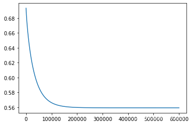
请注意等式中的"reg" 项。还注意到另外的一个“学习率”参数。这是一种超参数，用来控制正则化项。现在我们需要添加正则化梯度函数：

就像在第一部分中做的一样，初始化变量。

实验1 计算基于正则化得到的准确率

y_pred=[1 if item>=0.5 else 0  for item in sigmoid(X2@w).ravel()]
y_pred=np.array(y_pred)
np.sum(y_pred==y2)/y2.shape[0]

0.8305084745762712

现在，让我们尝试调用新的默认为0的 $w$ 的正则化函数，以确保计算工作正常。最后，我们可以使用第1部分中的预测函数来查看我们的方案在训练数据上的准确度。

2.8 试试sklearn

from sklearn import linear_model#调用sklearn的线性回归包
model = linear_model.LogisticRegression(penalty='l2', C=1.0)
model.fit(X2, y2.ravel())

LogisticRegression()

model.score(X2, y2)

0.8389830508474576

参考

[1] Andrew Ng. Machine Learning[EB/OL]. StanfordUniversity,2014.https://www.coursera.org/course/ml

[2] 李航. 统计学习方法[M]. 北京: 清华大学出版社,2019.

import sklearn.datasets as datasets
from sklearn.linear_model import LogisticRegression
import matplotlib.pyplot as plt

3.1 准备数据

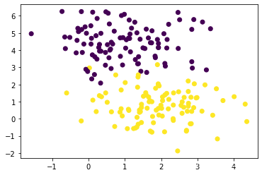
X, y = datasets.make_blobs(n_samples=200, n_features=2, centers=2, random_state=0)

X.shape, y.shape

((200, 2), (200,))

array([[ 2.8219307 ,  1.25395648],[ 1.65581849,  1.26771955],[ 3.12377692,  0.44427786],[ 1.4178305 ,  0.50039185],[ 2.50904929,  5.7731461 ],[ 0.30380963,  3.94423417],[ 1.12031365,  5.75806083],[ 0.08848433,  2.32299086],[ 1.92238694,  0.59987278],[-0.65392827,  4.76656958],[ 1.45895348,  0.84509636],[ 0.51447051,  0.96092565],[ 1.35269561,  3.20438654],[-0.27652528,  5.08127768],[ 2.15299249,  1.48061734],[ 0.17286041,  3.61423755],[-0.20029671, -0.12484318],[ 3.52184624,  1.7502156 ],[ 2.5763324 ,  0.32187569],[ 2.89689879,  0.64820508],[ 1.36742991, -0.31641374],[-0.33963733,  3.84220272],[ 2.07592967,  4.95905106],[ 0.206354  ,  4.84303652],[ 2.89921211,  5.78430212],[ 0.340424  ,  4.98022062],[ 1.78753398, -0.23034767],[ 1.18454506,  5.28042636],[ 1.61434489,  0.61730816],[-0.60390472,  1.50398318],[-0.19685333,  6.24740851],[ 0.72100905, -0.44905385],[ 2.96544643,  1.21488188],[ 1.06975678, -0.57417135],[ 0.90802847,  6.01713005],[-0.17119857,  3.86596728],[ 1.36321767,  2.43404071],[ 1.24190326, -0.56876067],[ 1.33263648,  5.0103605 ],[ 0.62835793,  4.4601363 ],[ 0.70826671,  5.10624372],[ 2.8285205 , -0.28621698],[ 1.57561171,  1.51802196],[ 0.94808785,  4.7321192 ],[ 1.0427873 ,  4.60625923],[ 2.19722068,  0.57833524],[-0.29421492,  5.27318404],[ 0.02458305,  2.96215652],[ 2.16429987,  4.62072994],[ 4.31457647,  0.85540651],[ 0.86640826,  0.39084731],[ 1.5528609 ,  4.09548857],[ 1.44193252,  2.76754364],[ 0.93698726,  3.13569383],[ 2.21177406,  1.1298447 ],[ 0.46546494,  3.12315514],[ 3.13950603,  5.64031528],[ 0.9867701 ,  6.08965782],[ 1.74438135,  0.99506383],[ 0.89791226,  0.58537141],[ 2.74904067,  0.73809022],[ 4.01117983,  1.28775698],[-0.09448254,  5.35823905],[ 0.62227617,  2.92883603],[ 3.35941485,  5.24826681],[ 2.1047625 ,  1.39150044],[ 1.01001416,  2.10880895],[ 2.63378902,  1.24731812],[ 2.15504965,  4.12386249],[ 0.28170222,  4.15415279],[ 4.35918422, -0.16235216],[ 0.4666179 ,  3.86571303],[ 0.11898772,  1.08644226],[ 1.69057398,  1.05436752],[ 1.92156596,  1.97540747],[ 2.84159548,  0.43124456],[ 1.89760051,  3.15438716],[ 0.74874067,  2.55579434],[ 0.1631238 ,  2.57750473],[ 1.45661358, -0.21823333],[ 1.14294357,  4.93881876],[ 2.03824711,  1.2768154 ],[-1.57671974,  4.95740592],[-0.73000011,  6.25456272],[ 1.37125662,  2.55721446],[ 2.84382904,  5.20983199],[-0.51498751,  4.74317903],[ 2.01309607,  0.61077647],[ 1.67038771,  0.99201525],[ 1.59167155,  1.37914513],[ 1.37861172,  3.61897724],[-0.02394527,  2.75901623],[ 0.11504439,  6.21385228],[ 2.11567076,  3.06896151],[ 1.91931782,  2.03455502],[ 2.03958541,  1.05859183],[ 1.84836385,  1.77784257],[ 0.52073758,  4.32126649],[ 1.0220286 ,  4.11660348],[ 1.2911236 , -0.54012781],[ 0.34194798,  3.94104616],[ 2.5490093 ,  0.78155972],[ 1.15369622,  3.90200639],[ 0.60708824,  4.06440815],[-0.63762777,  4.09104705],[ 1.28933778,  3.44969159],[-0.12811326,  4.35595241],[ 0.08080352,  4.69068983],[ 3.20759909,  1.97728225],[ 0.06344785,  5.42080362],[ 2.80245586, -0.2912813 ],[ 2.20656076,  5.50616718],[ 1.7373078 ,  4.42546234],[ 1.70536064,  4.43277024],[ 0.47823763,  6.23331938],[ 2.6225578 ,  0.67498856],[ 0.21219797,  0.41968966],[ 1.76343016,  0.13617145],[ 1.09932252,  0.55168188],[ 1.86461403,  0.50281415],[ 1.59034945,  5.225994  ],[ 2.48152625,  1.57457169],[ 0.58894326,  4.00148458],[ 1.35056725,  1.84092438],[ 0.3571617 ,  1.28494414],[ 2.7216506 ,  0.43694387],[ 1.92352205,  4.14877723],[ 2.0309414 ,  0.15963275],[ 2.69858199, -0.67295975],[ 1.83310069,  3.65276173],[ 1.45795145,  0.65974193],[ 1.37227679,  3.21072582],[ 0.54111653,  6.15305106],[ 2.57915855,  0.98608575],[ 0.23151526,  3.47734879],[ 2.84382807,  3.32650945],[-0.24916544,  5.1481503 ],[ 1.40285894,  0.50671028],[ 2.74508569,  2.19950989],[ 3.70340245,  1.06189142],[ 1.42013331,  4.63746165],[ 0.47232912,  1.50804304],[ 1.8971289 ,  4.62251498],[ 0.10547293,  3.72493766],[ 2.32978388,  0.00674858],[ 1.60150153,  2.70172967],[ 0.30193742,  4.33561789],[-0.31658683,  4.5708382 ],[ 2.34161121,  1.50650749],[ 1.94472686,  1.91783637],[ 1.40297392,  0.37647435],[ 0.06897171,  4.35573272],[ 1.74806063,  5.12729148],[ 1.49954674,  4.132241  ],[ 0.63120661,  0.40434378],[ 1.27450825,  5.63017322],[ 0.66471755,  4.35995267],[ 1.42717996,  0.41663654],[ 2.9871159 ,  1.23762864],[ 1.33566313,  0.08467067],[ 0.92844171,  0.16698591],[ 2.46452227,  6.1996765 ],[ 2.85942078,  2.95602827],[ 2.69539905, -0.71929238],[ 1.70183577, -0.71881053],[ 1.11082127,  0.48761397],[ 0.23670708,  5.84680192],[ 1.1312175 ,  4.68194985],[ 0.33265168,  2.08038418],[-0.07228289,  2.88376939],[ 1.74625455, -0.77834015],[ 1.93710348,  0.21748546],[ 3.41979937,  0.20821448],[ 1.10318217,  4.70577669],[ 2.33570923, -0.09545995],[ 1.64856484,  4.71124916],[ 1.92569089,  4.39133857],[ 0.57309313,  5.5262324 ],[ 3.54975207, -1.17232137],[ 2.45431387, -1.8749291 ],[ 0.89908509,  1.67886176],[ 1.84070628,  3.56162231],[ 1.99364112,  0.79035838],[ 2.102906  ,  3.22385582],[ 0.87305123,  4.71438583],[ 0.5626511 ,  3.55633252],[ 2.75372467,  0.90143455],[ 2.09389807, -0.75905144],[ 1.32967014, -0.4857003 ],[-0.05797276,  4.98538185],[ 1.51240605,  1.31371371],[ 0.87781755,  3.64030904],[ 0.29937694,  1.34859812],[ 2.33519212,  0.79951327],[ 2.91319145,  2.03876553],[ 2.74680627,  1.5924128 ],[ 2.47034915,  4.09862906],[ 3.2460247 ,  2.84942165],[ 1.9263585 ,  4.15243012],[-0.18887976,  5.20461381]])

plt.scatter(X[:, 0], X[:, 1], c=y)

<matplotlib.collections.PathCollection at 0x142327368e0>

实验2 完成3.2 调用逻辑回归模型完成分类

3.2 调用普通的逻辑回归模型来进行多分类(调用1.4的梯度下降算法)

X=np.insert(X,0,1,axis=1)
X

array([[ 1.        ,  2.8219307 ,  1.25395648],[ 1.        ,  1.65581849,  1.26771955],[ 1.        ,  3.12377692,  0.44427786],[ 1.        ,  1.4178305 ,  0.50039185],[ 1.        ,  2.50904929,  5.7731461 ],[ 1.        ,  0.30380963,  3.94423417],[ 1.        ,  1.12031365,  5.75806083],[ 1.        ,  0.08848433,  2.32299086],[ 1.        ,  1.92238694,  0.59987278],[ 1.        , -0.65392827,  4.76656958],[ 1.        ,  1.45895348,  0.84509636],[ 1.        ,  0.51447051,  0.96092565],[ 1.        ,  1.35269561,  3.20438654],[ 1.        , -0.27652528,  5.08127768],[ 1.        ,  2.15299249,  1.48061734],[ 1.        ,  0.17286041,  3.61423755],[ 1.        , -0.20029671, -0.12484318],[ 1.        ,  3.52184624,  1.7502156 ],[ 1.        ,  2.5763324 ,  0.32187569],[ 1.        ,  2.89689879,  0.64820508],[ 1.        ,  1.36742991, -0.31641374],[ 1.        , -0.33963733,  3.84220272],[ 1.        ,  2.07592967,  4.95905106],[ 1.        ,  0.206354  ,  4.84303652],[ 1.        ,  2.89921211,  5.78430212],[ 1.        ,  0.340424  ,  4.98022062],[ 1.        ,  1.78753398, -0.23034767],[ 1.        ,  1.18454506,  5.28042636],[ 1.        ,  1.61434489,  0.61730816],[ 1.        , -0.60390472,  1.50398318],[ 1.        , -0.19685333,  6.24740851],[ 1.        ,  0.72100905, -0.44905385],[ 1.        ,  2.96544643,  1.21488188],[ 1.        ,  1.06975678, -0.57417135],[ 1.        ,  0.90802847,  6.01713005],[ 1.        , -0.17119857,  3.86596728],[ 1.        ,  1.36321767,  2.43404071],[ 1.        ,  1.24190326, -0.56876067],[ 1.        ,  1.33263648,  5.0103605 ],[ 1.        ,  0.62835793,  4.4601363 ],[ 1.        ,  0.70826671,  5.10624372],[ 1.        ,  2.8285205 , -0.28621698],[ 1.        ,  1.57561171,  1.51802196],[ 1.        ,  0.94808785,  4.7321192 ],[ 1.        ,  1.0427873 ,  4.60625923],[ 1.        ,  2.19722068,  0.57833524],[ 1.        , -0.29421492,  5.27318404],[ 1.        ,  0.02458305,  2.96215652],[ 1.        ,  2.16429987,  4.62072994],[ 1.        ,  4.31457647,  0.85540651],[ 1.        ,  0.86640826,  0.39084731],[ 1.        ,  1.5528609 ,  4.09548857],[ 1.        ,  1.44193252,  2.76754364],[ 1.        ,  0.93698726,  3.13569383],[ 1.        ,  2.21177406,  1.1298447 ],[ 1.        ,  0.46546494,  3.12315514],[ 1.        ,  3.13950603,  5.64031528],[ 1.        ,  0.9867701 ,  6.08965782],[ 1.        ,  1.74438135,  0.99506383],[ 1.        ,  0.89791226,  0.58537141],[ 1.        ,  2.74904067,  0.73809022],[ 1.        ,  4.01117983,  1.28775698],[ 1.        , -0.09448254,  5.35823905],[ 1.        ,  0.62227617,  2.92883603],[ 1.        ,  3.35941485,  5.24826681],[ 1.        ,  2.1047625 ,  1.39150044],[ 1.        ,  1.01001416,  2.10880895],[ 1.        ,  2.63378902,  1.24731812],[ 1.        ,  2.15504965,  4.12386249],[ 1.        ,  0.28170222,  4.15415279],[ 1.        ,  4.35918422, -0.16235216],[ 1.        ,  0.4666179 ,  3.86571303],[ 1.        ,  0.11898772,  1.08644226],[ 1.        ,  1.69057398,  1.05436752],[ 1.        ,  1.92156596,  1.97540747],[ 1.        ,  2.84159548,  0.43124456],[ 1.        ,  1.89760051,  3.15438716],[ 1.        ,  0.74874067,  2.55579434],[ 1.        ,  0.1631238 ,  2.57750473],[ 1.        ,  1.45661358, -0.21823333],[ 1.        ,  1.14294357,  4.93881876],[ 1.        ,  2.03824711,  1.2768154 ],[ 1.        , -1.57671974,  4.95740592],[ 1.        , -0.73000011,  6.25456272],[ 1.        ,  1.37125662,  2.55721446],[ 1.        ,  2.84382904,  5.20983199],[ 1.        , -0.51498751,  4.74317903],[ 1.        ,  2.01309607,  0.61077647],[ 1.        ,  1.67038771,  0.99201525],[ 1.        ,  1.59167155,  1.37914513],[ 1.        ,  1.37861172,  3.61897724],[ 1.        , -0.02394527,  2.75901623],[ 1.        ,  0.11504439,  6.21385228],[ 1.        ,  2.11567076,  3.06896151],[ 1.        ,  1.91931782,  2.03455502],[ 1.        ,  2.03958541,  1.05859183],[ 1.        ,  1.84836385,  1.77784257],[ 1.        ,  0.52073758,  4.32126649],[ 1.        ,  1.0220286 ,  4.11660348],[ 1.        ,  1.2911236 , -0.54012781],[ 1.        ,  0.34194798,  3.94104616],[ 1.        ,  2.5490093 ,  0.78155972],[ 1.        ,  1.15369622,  3.90200639],[ 1.        ,  0.60708824,  4.06440815],[ 1.        , -0.63762777,  4.09104705],[ 1.        ,  1.28933778,  3.44969159],[ 1.        , -0.12811326,  4.35595241],[ 1.        ,  0.08080352,  4.69068983],[ 1.        ,  3.20759909,  1.97728225],[ 1.        ,  0.06344785,  5.42080362],[ 1.        ,  2.80245586, -0.2912813 ],[ 1.        ,  2.20656076,  5.50616718],[ 1.        ,  1.7373078 ,  4.42546234],[ 1.        ,  1.70536064,  4.43277024],[ 1.        ,  0.47823763,  6.23331938],[ 1.        ,  2.6225578 ,  0.67498856],[ 1.        ,  0.21219797,  0.41968966],[ 1.        ,  1.76343016,  0.13617145],[ 1.        ,  1.09932252,  0.55168188],[ 1.        ,  1.86461403,  0.50281415],[ 1.        ,  1.59034945,  5.225994  ],[ 1.        ,  2.48152625,  1.57457169],[ 1.        ,  0.58894326,  4.00148458],[ 1.        ,  1.35056725,  1.84092438],[ 1.        ,  0.3571617 ,  1.28494414],[ 1.        ,  2.7216506 ,  0.43694387],[ 1.        ,  1.92352205,  4.14877723],[ 1.        ,  2.0309414 ,  0.15963275],[ 1.        ,  2.69858199, -0.67295975],[ 1.        ,  1.83310069,  3.65276173],[ 1.        ,  1.45795145,  0.65974193],[ 1.        ,  1.37227679,  3.21072582],[ 1.        ,  0.54111653,  6.15305106],[ 1.        ,  2.57915855,  0.98608575],[ 1.        ,  0.23151526,  3.47734879],[ 1.        ,  2.84382807,  3.32650945],[ 1.        , -0.24916544,  5.1481503 ],[ 1.        ,  1.40285894,  0.50671028],[ 1.        ,  2.74508569,  2.19950989],[ 1.        ,  3.70340245,  1.06189142],[ 1.        ,  1.42013331,  4.63746165],[ 1.        ,  0.47232912,  1.50804304],[ 1.        ,  1.8971289 ,  4.62251498],[ 1.        ,  0.10547293,  3.72493766],[ 1.        ,  2.32978388,  0.00674858],[ 1.        ,  1.60150153,  2.70172967],[ 1.        ,  0.30193742,  4.33561789],[ 1.        , -0.31658683,  4.5708382 ],[ 1.        ,  2.34161121,  1.50650749],[ 1.        ,  1.94472686,  1.91783637],[ 1.        ,  1.40297392,  0.37647435],[ 1.        ,  0.06897171,  4.35573272],[ 1.        ,  1.74806063,  5.12729148],[ 1.        ,  1.49954674,  4.132241  ],[ 1.        ,  0.63120661,  0.40434378],[ 1.        ,  1.27450825,  5.63017322],[ 1.        ,  0.66471755,  4.35995267],[ 1.        ,  1.42717996,  0.41663654],[ 1.        ,  2.9871159 ,  1.23762864],[ 1.        ,  1.33566313,  0.08467067],[ 1.        ,  0.92844171,  0.16698591],[ 1.        ,  2.46452227,  6.1996765 ],[ 1.        ,  2.85942078,  2.95602827],[ 1.        ,  2.69539905, -0.71929238],[ 1.        ,  1.70183577, -0.71881053],[ 1.        ,  1.11082127,  0.48761397],[ 1.        ,  0.23670708,  5.84680192],[ 1.        ,  1.1312175 ,  4.68194985],[ 1.        ,  0.33265168,  2.08038418],[ 1.        , -0.07228289,  2.88376939],[ 1.        ,  1.74625455, -0.77834015],[ 1.        ,  1.93710348,  0.21748546],[ 1.        ,  3.41979937,  0.20821448],[ 1.        ,  1.10318217,  4.70577669],[ 1.        ,  2.33570923, -0.09545995],[ 1.        ,  1.64856484,  4.71124916],[ 1.        ,  1.92569089,  4.39133857],[ 1.        ,  0.57309313,  5.5262324 ],[ 1.        ,  3.54975207, -1.17232137],[ 1.        ,  2.45431387, -1.8749291 ],[ 1.        ,  0.89908509,  1.67886176],[ 1.        ,  1.84070628,  3.56162231],[ 1.        ,  1.99364112,  0.79035838],[ 1.        ,  2.102906  ,  3.22385582],[ 1.        ,  0.87305123,  4.71438583],[ 1.        ,  0.5626511 ,  3.55633252],[ 1.        ,  2.75372467,  0.90143455],[ 1.        ,  2.09389807, -0.75905144],[ 1.        ,  1.32967014, -0.4857003 ],[ 1.        , -0.05797276,  4.98538185],[ 1.        ,  1.51240605,  1.31371371],[ 1.        ,  0.87781755,  3.64030904],[ 1.        ,  0.29937694,  1.34859812],[ 1.        ,  2.33519212,  0.79951327],[ 1.        ,  2.91319145,  2.03876553],[ 1.        ,  2.74680627,  1.5924128 ],[ 1.        ,  2.47034915,  4.09862906],[ 1.        ,  3.2460247 ,  2.84942165],[ 1.        ,  1.9263585 ,  4.15243012],[ 1.        , -0.18887976,  5.20461381]])

#调用梯度下降算法
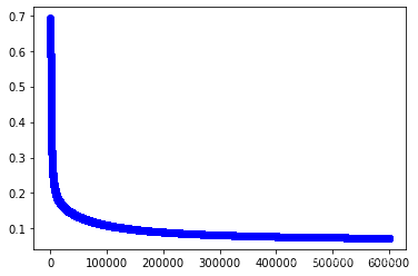
iter_num,alpha=600000,0.001
w,cost_lst=grandient(X,y,iter_num,alpha)

#绘制误差曲线
plt.plot(range(iter_num),cost_lst,"b-o")

[<matplotlib.lines.Line2D at 0x1423849dc70>]

X[y==0,1]

array([ 2.50904929,  0.30380963,  1.12031365,  0.08848433, -0.65392827,1.35269561, -0.27652528,  0.17286041, -0.33963733,  2.07592967,0.206354  ,  2.89921211,  0.340424  ,  1.18454506, -0.19685333,0.90802847, -0.17119857,  1.33263648,  0.62835793,  0.70826671,0.94808785,  1.0427873 , -0.29421492,  2.16429987,  1.5528609 ,1.44193252,  0.93698726,  0.46546494,  3.13950603,  0.9867701 ,-0.09448254,  0.62227617,  3.35941485,  2.15504965,  0.28170222,0.4666179 ,  0.1631238 ,  1.14294357, -1.57671974, -0.73000011,2.84382904, -0.51498751,  1.37861172, -0.02394527,  0.11504439,2.11567076,  0.52073758,  1.0220286 ,  0.34194798,  1.15369622,0.60708824, -0.63762777,  1.28933778, -0.12811326,  0.08080352,0.06344785,  2.20656076,  1.7373078 ,  1.70536064,  0.47823763,1.59034945,  0.58894326,  1.92352205,  1.83310069,  1.37227679,0.54111653,  0.23151526,  2.84382807, -0.24916544,  1.42013331,1.8971289 ,  0.10547293,  1.60150153,  0.30193742, -0.31658683,0.06897171,  1.74806063,  1.49954674,  1.27450825,  0.66471755,2.46452227,  2.85942078,  0.23670708,  1.1312175 ,  0.33265168,-0.07228289,  1.10318217,  1.64856484,  1.92569089,  0.57309313,1.84070628,  2.102906  ,  0.87305123,  0.5626511 , -0.05797276,0.87781755,  2.47034915,  3.2460247 ,  1.9263585 , -0.18887976])

#绘制线性的决策边界
x_exmal=np.linspace(np.min(X[:,1]),np.max(X[:,1]),50)
x2=(-w[0,0]-w[1,0]*x_exmal)/(w[2,0])
plt.plot(x_exmal,x2,"r-o")
plt.scatter(X[y==1,1],X[y==1,2],color="b",marker="o")
plt.scatter(X[y==0,1],X[y==0,2],color="c",marker="^")
plt.show()

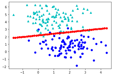
#计算准确率
y_pred=[1 if item>=0.5 else 0  for item in sigmoid(X@w).ravel()]
y_pred=np.array(y_pred)
np.sum(y_pred==y)/y.shape[0]

0.97

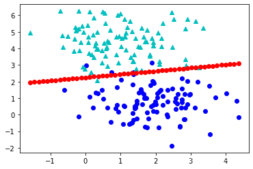
实验3 完成3.3 调用正则化的逻辑回归模型完成分类

3.3调用正则化的逻辑回归模型来进行多分类(调用2.7的梯度下降算法)

y.shape,X.shape,w.shape

((200,), (200, 3), (3, 1))

#调用梯度下降算法
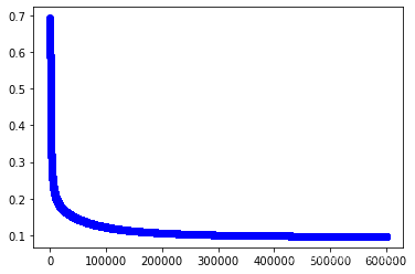
iter_num,alpha,lambd=600000,0.001,1
w,cost_lst=grandient_reg(X,w,y,iter_num,alpha,lambd)

#绘制误差曲线
plt.plot(range(iter_num),cost_lst,"b-o")

[<matplotlib.lines.Line2D at 0x1423279f070>]

#绘制线性的决策边界
x_exmal=np.linspace(np.min(X[:,1]),np.max(X[:,1]),50)
x2=(-w[0,0]-w[1,0]*x_exmal)/(w[2,0])
plt.plot(x_exmal,x2,"r-o")
plt.scatter(X[y==1,1],X[y==1,2],color="b",marker="o")
plt.scatter(X[y==0,1],X[y==0,2],color="c",marker="^")
plt.show()

y.shape,X.shape,w.shape

((200,), (200, 3), (3, 1))

#计算准确率
y_pred=[1 if item>=0.5 else 0  for item in sigmoid(X@w).ravel()]
y_pred=np.array(y_pred)
np.sum(y_pred==y)/y.shape[0]

0.97

实验4 完成3.3 调用SKLEARN完成分类

3.4 调用SKLEARN

from sklearn.linear_model import LogisticRegression
clf = LogisticRegression().fit(X, y)
clf.score(X,y)

0.97

【Python机器学习】实验03 logstic回归