1. 安装与入门

1.1 python封装

安装pip install elkai
使用时需传入距离矩阵，例如：

import numpy as np
import elkaiM = np.zeros((3, 3), dtype=int)
M[0, 1] = 4
M[1, 2] = 5print(elkai.solve_int_matrix(M)) # 可以传入runs=10参数
# Output: [0, 2, 1]

1.2 原版

原版地址见http://akira.ruc.dk/~keld/research/LKH-3/
git镜像地址为https://github.com/cerebis/LKH3
最新的版本是3.0.7，下载地址为http://akira.ruc.dk/~keld/research/LKH-3/LKH-3.0.7.tgz，解压并编译：

tar xvfz LKH-3.0.7.tgz
cd LKH-3.0.7
make

对于windows用户，下载地址：http://akira.ruc.dk/~keld/research/LKH-3/LKH-3.exe

首先需要一个tsp文件，然后需要一个par文件，里面的内容参考如下：

PROBLEM_FILE = pr2392.tsp
#OPTIMUM = 378032
#MOVE_TYPE = 5
#PATCHING_C = 3
#PATCHING_A = 2
#RUNS = 10

PROBLEM_FILE是必须要有的。
官方示例文件如下：
在这里插入图片描述

我们使用pr2392来测试./LKH pr2392.par
观察一下输出：

Lower bound = 373488.5, Gap = 1.20%, Ascent time = 5.31 sec.
Cand.min = 2, Cand.avg = 5.0, Cand.max = 5
Preprocessing time = 5.46 sec.
* 1: Cost = 378224, Gap = 0.0508%, Time = 0.28 sec.
* 2: Cost = 378032, Gap = 0.0000%, Time = 0.36 sec. =
Run 1: Cost = 378032, Gap = 0.0000%, Time = 0.36 sec. =
...
Cost.min = 378032, Cost.avg = 378032.00, Cost.max = 378032
Gap.min = 0.0000%, Gap.avg = 0.0000%, Gap.max = 0.0000%
Trials.min = 1, Trials.avg = 5.8, Trials.max = 29
Time.min = 0.24 sec., Time.avg = 0.51 sec., Time.max = 1.06 sec.
Time.total = 10.61 sec.

2. 核心概念

2.1 sequential exchange

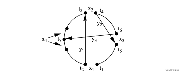
x是要取消的边，y是要添加的边，下标编号规则如下：
在这里插入图片描述
令break的边标号为x1,x2,…，repair的边标号y1,y2,…，如下图所示：

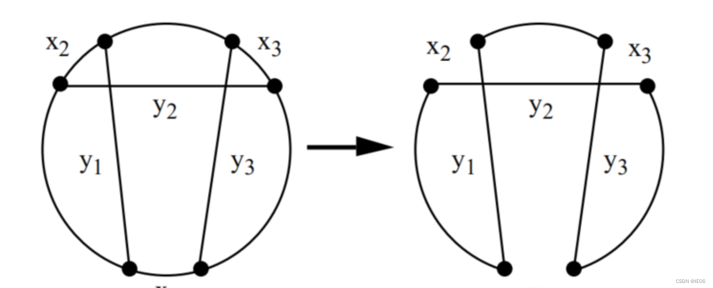
满足如下规则：

序列（x1，y1，x2，y2，…，xr，yr）构成了一条邻近的链路
任意i>=3，有xi和x1能够闭合（形成yr）
G+=xi-yi永远为正数

2.2 close up

当 $x_2$ 的末端 $t_4$ 与 $t_1$ 连接后产生subtour，则称 $x_2$ 打破close up。
在这里插入图片描述
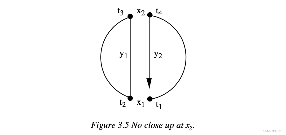
我们只允许 $x_2$ 打破close up，往后就不允许了。例如 $y_2$ 往左后，接下来两个 $x_3$ 都能close up。

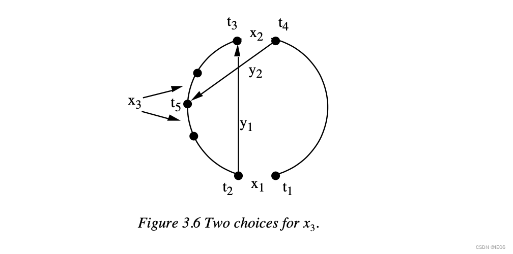
但是如果 $y_2$ 向右边探索的话， $x_3$ 就只能往上走，否则会出现 $t_5$ 、 $t_4$ 会形成subtour。

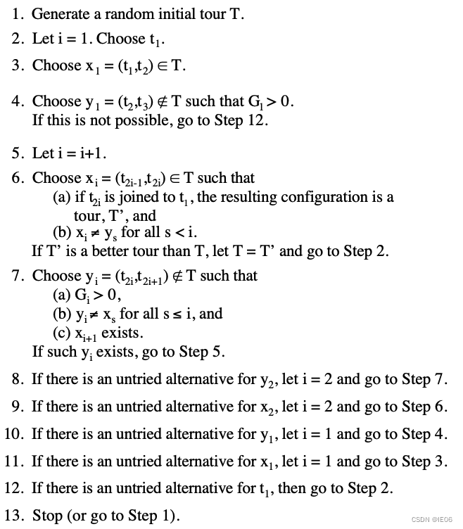
2.3 backtracking

遍历只发生在 $i = 1, 2$ ，也就是 $x_1,x_2,y_1,y_2$ 上。如下流程图，8-12就是backtracking。
在这里插入图片描述

2.4 α-measure

首先定义1-tree：
在这里插入图片描述

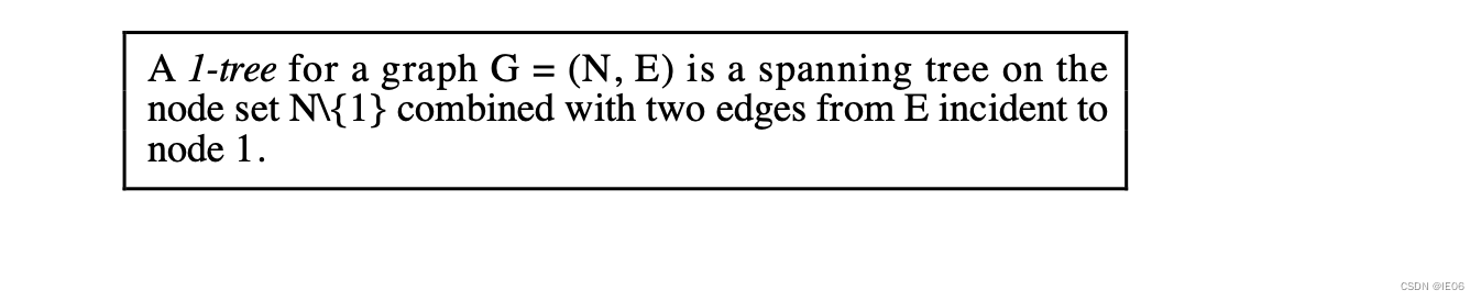
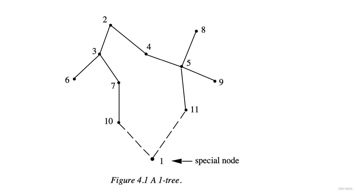
简单来说，就是去掉special node以及其连接的两条边后，剩下的边构成生成树。
接下来定义α-measure：

我们的candidate set，包含了k个α-nearest边，或者是包含了α-nearness小于一定值的边。
算法会用 {2, 3, …, n}构建一个最小生成树（可以使用prim算法），然后加上与1最近的两个点形成的边，得到T
然后计算所有边的α(i,j) ，确定方法为：

如果(i,j)属于T，则 $T^+(i,j)=T$
如果(i,j)包含1，比如说 $i = 1$ ，则将T中与1相连的两条边(1,a)与(1,b)中较长的那个换成 $(1, j)$ 即可
否则将(i,j)插入T中，在形成的环中，删除最长的一条边即可。
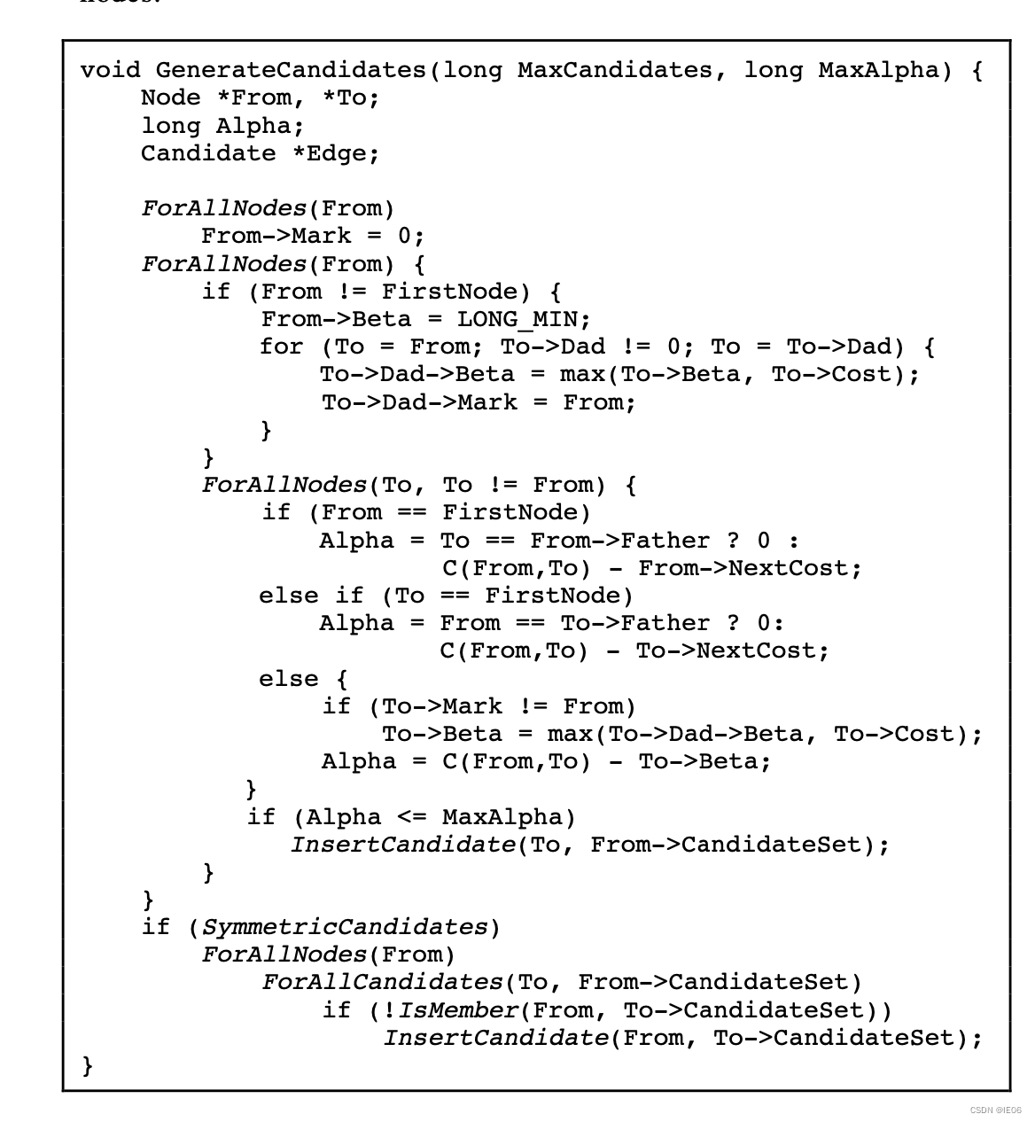
我们可以用递推关系式来进行计算。令α(i,j)=c(i,j)-β(i,j) ，即β是添加(i,j)后需要删掉的边的长度，我们有β(i,j2) = max( β(i,j1) ,c(j1,j2)).

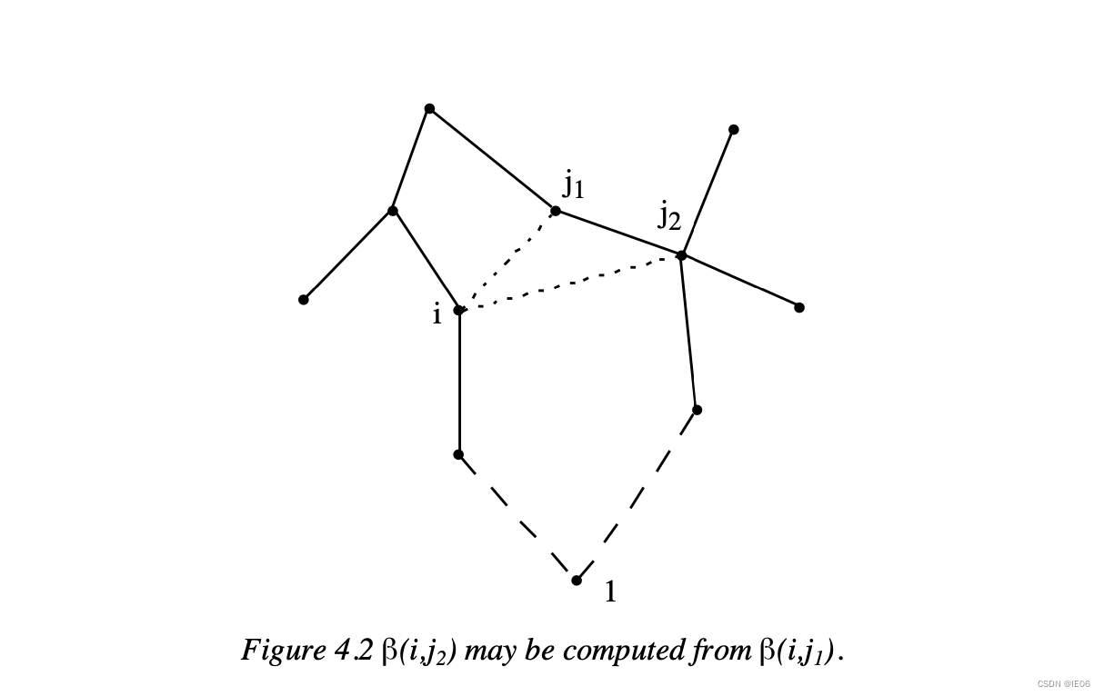
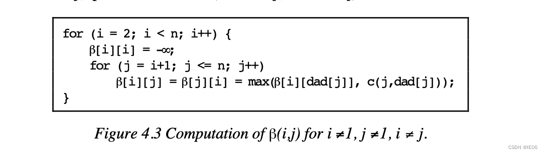
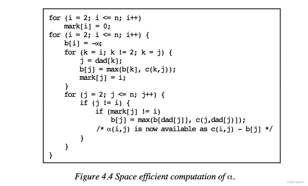
节省空间的一个算法如下，令b[j] = [β[i,j]…]。首先计算从i到根节点的路径上的b，再计算剩下节点的b即可（使用mark辅助，排除已经计算过的边）。

2.5 π值

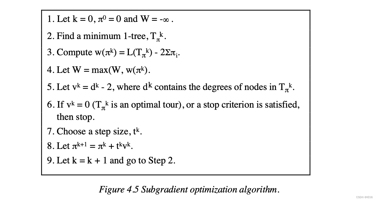
我们令 $d_{ij} = c_{ij} + π_i + π_j$ ，则最优解是不变的，但是minimum 1-tree会变。令 $T_π$ 为新的距离矩阵上的最小1-tree， $L(T_π)$ 为其总距离，我们希望最大化 $w(π)=L(T_π)-2Σπ_i$ ，然后我们就可以用这个最大值作为lower bound了。
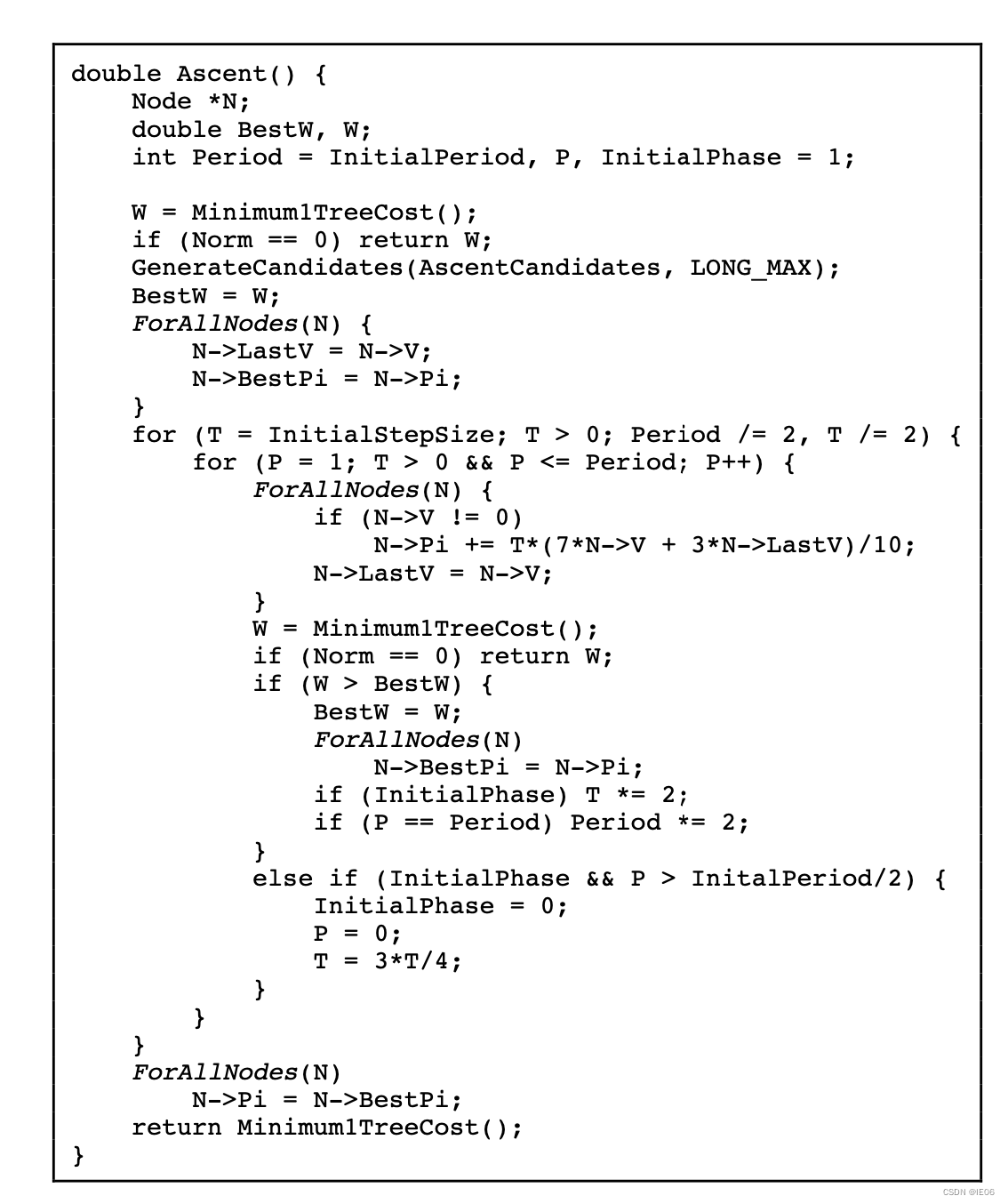
寻找 $π_i$ 的方法是使用梯度下降法，从 $π^0=$ [0,0…0]开始， $π^{k+1} = π^k + t^kv^k$ ，t是step size。这里我们令 $v^k = d^k - 2$ ，其中 $d^k$ 是当前节点的degree。算法如下：
在这里插入图片描述

下面是关于step size的启发式规则：

在period(=n/2)期间内，从 $t^0=1$ 开始，逐步*2直至W不再增长，随后保持这个数据直至period结束。
如果直至period结束还在增长，则将period*2继续。
随后period/2， $t^1=t^0/2$ 继续下一轮迭代
同理迭代，直至period、t、v其中有一个变为0.
另外还有一个修改

这是3种方案的对比：

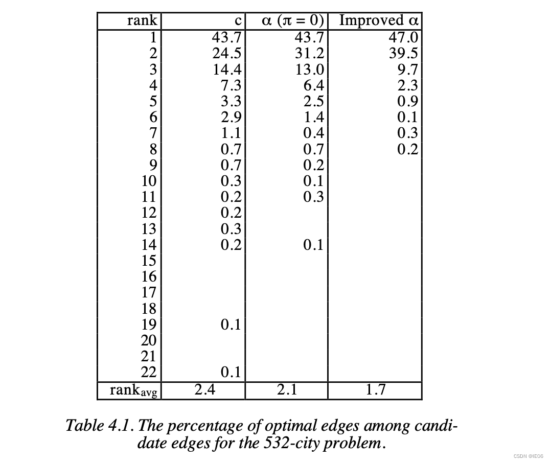
2.6 initial tour

算法如下：
在这里插入图片描述
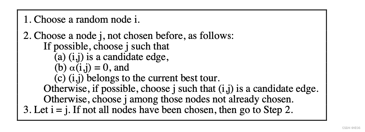
概述：从任意一点出发，逐步构造出完整的路径。每次走向下一个点时，尽量选择candidate edge。

3. 代码分析

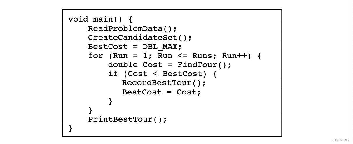
3.1 总体流程

调试时的配置如下：
在这里插入图片描述
整体流程如下：

3.2 创建candidate sets

其中candidate set基于α-nearness建立。
在这里插入图片描述
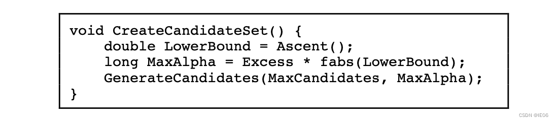
Ascent使用梯度下降法给出lowerbound以及最佳的π
Excess是一个比例，乘以lowerbound后得到MaxAlpha，用来控制α-nearness的最大值
MaxCandidates则是每个点允许的最大candidates数目。
其中Ascent部分代码如下，其中Norm=L2(v-value)，可以看做是损失函数
在这里插入图片描述
根据π得到candidates的代码如下，里面大部分是计算α-nearness的代码。candidate set包含了α-nearness小于MaxAlpha的边，体现在InsertCandidate函数中。

3.3 find tour

总体框架如图：
在这里插入图片描述
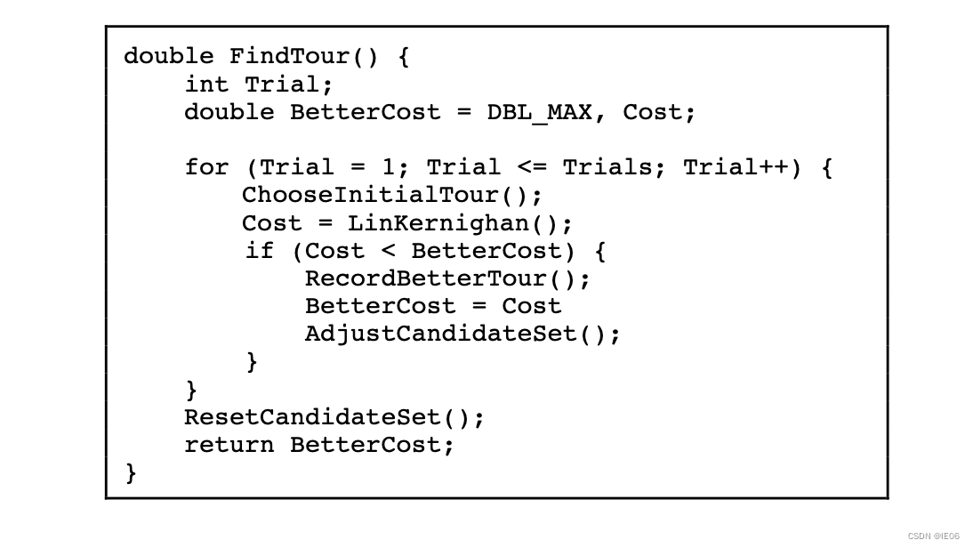
其中核心函数LinKernighan如下，遍历所有的x1=(t1,t2)寻找better tour：

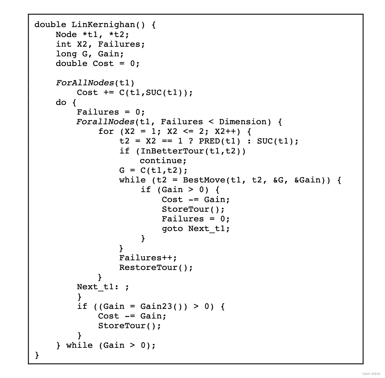
其中BestMove默认使用5-opt算子：

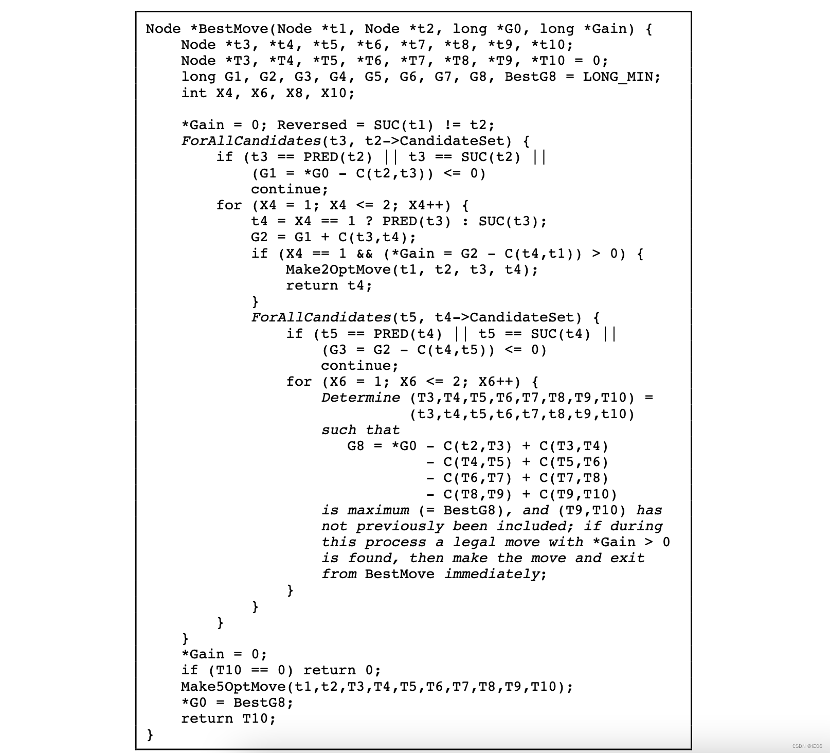
一共需要break和repair5条边，其中x1=(t1,t2)是遍历所有边，y1=(t2,t3)遍历所有t2的CandidateSet。如果G1<=0，则直接继续下一次搜索。
一旦选好t3，那么x2=(t3,t4)有向前向后两种选择。如果连接(t4,t1)后的Gain得到优化，那么直接进行2-opt边交换操作，并跳出循环；否则y2=(t4,t5)遍历所有t4的CandidateSet。如果G3<=0，则直接继续下一次搜索。
选好t5后，同理往下，继续选择x3,y3,x4,y4,x5。这时如果连接(t10,t1)后的Gain得到优化，那么进行边交换并退出循环。

3.4 don’t look bit

每一个点都设置了一个don’t look bit，初始化为0.每当t1的improving move失败，会将t1的bit设置为1；如果成功，则会将其设置为0.
在遍历t1时，所有bit为1的点都会跳过。

3.5 参数文件

RUNS =
The total number of runs. Default: 10.

MAX_TRIALS =
The maximum number of trials in each run.
Default: number of nodes (DIMENSION, given in the problem file).

TOUR_FILE =
Specifies the name of a file to which the best tour is to be written.

OPTIMUM =
Known optimal tour length. A run will be terminated as soon as a tour length less than or equal to optimum is achieved.
Default: DBL_MAX.

MAX_CANDIDATES = { SYMMETRIC }
The maximum number of candidate edges to be associated with each node.
The integer may be followed by the keyword SYMMETRIC, signifying that the candidate set is to be complemented such that every candidate edge is associated with both its two end nodes.
Default: 5.

ASCENT_CANDIDATES =
The number of candidate edges to be associated with each node during the ascent. The candidate set is complemented such that every candidate edge is associated with both its two end nodes.
Default: 50.

EXCESS =
The maximum α-value allowed for any candidate edge is set to EXCESS times the absolute value of the lower bound of a solution tour (determined by the ascent). Default: 1.0/DIMENSION.

INITIAL_PERIOD =
The length of the first period in the ascent. Default: DIMENSION/2 (but at least 100).

INITIAL_STEP_SIZE =
The initial step size used in the ascent. Default: 1.

PI_FILE =
Specifies the name of a file to which penalties (π-values determined by the ascent) is to be written. If the file already exits, the penalties are read from the file, and the ascent is skipped.

PRECISION =
The internal precision in the representation of transformed distances: dij = PRECISION*cij + πi + πj, where dij, cij, πi and πj are all integral.
Default: 100 (which corresponds to 2 decimal places).

SEED =
Specifies the initial seed for random number generation. Default: 1.

SUBGRADIENT: [ YES | NO ]
Specifies whether the π-values should be determined by subgradient optimization. Default: YES.

TRACE_LEVEL =
Specifies the level of detail of the output given during the solution process. The value 0 signifies a minimum amount of output. The higher the value is the more information is given.
Default: 1.

3.6 数据结构

swap指一次2-opt交换。
最基本的数据结构是double linked list，rank给出的是在tour中的排序。
在这里插入图片描述
为了加快2-opt交换，还设计了一种two-level tree结构，rank给出的是在segment中的排序

segment的数据结构如下，rank给出的是segment在总的tour中的排序，first和last是segment的第一个节点和最后一个节点的标记。