2018 Atrial Segmentation Challenge
数据准备
The Left Atrium (LA) MR dataset from the Atrial Segmentation Challenge
数据集下载地址:Data – 2018 Atrial Segmentation Challenge (cardiacatlas.org)

数据集结构:
Training_Set
├── 0RZDK210BSMWAA6467LU
│   ├── laendo.nrrd
│   └── lgemri.nrrd
├── 1D7CUD1955YZPGK8XHJX
│   ├── laendo.nrrd
│   └── lgemri.nrrd
......
Testing_Set
├── 4URSJYI2QUH1T5S5PP47
│   ├── laendo.nrrd
│   └── lgemri.nrrd
├── 6HDYMTGBRI27MN763XTS
│   ├── laendo.nrrd
│   └── lgemri.nrrd
......
- 一共有154例包含心房颤动的 3D MRI 图像
- 分为训练集(Training Set)和测试集(Testing Set,已开源),数据集下每个文件夹包含一个患者的MRI(lgemri.nrrd)和标签图像(laendo.nrrd)
- MRI灰度分布在[0, 255],空间分辨率为 0.625 x 0.625 x 0.625 mm³,切片尺寸因人而异,Z轴包含88个切片
- 标签为二值图,0代表背景,255代表分割区域(左心房)
数据处理
所有的MRI数据空间分辨率都为 0.625 x 0.625 x 0.625 mm³,因此不需要做重采样。灰度分布都在0~255之间,也不需要做约束。
首先,将训练集和测试集放在一个文件夹里面,统一进行处理。
做三维图像的数据处理之前,最好提前确定目标尺寸,就是你输入到神经网络中的图像尺寸。可以用3D slicer提前看一下,分割区域大致有多大,选定的尺寸至少要包含目标区域。我选定的目标尺寸是 112 x 112 x 80,裁剪的时候不要一步裁剪到了目标尺寸,可以裁剪的比 112 x 112 x 80 略大,这样我们在做数据增强的时候,才能保证空间上的多样性,比如说平移。
具体操作可以看代码:
- data_path 为合并后的数据集地址,包含 154 对图像
- out_path 是输出地址,保存裁剪后的数据
import os
import numpy as np
from tqdm import tqdm
import h5py
import nrrdoutput_size =[112, 112, 80]
data_path = 'E:/data/LASet/origin'
out_path = 'E:/data/LASet/data'
def covert_h5():listt = os.listdir(data_path)for case in tqdm(listt):image, img_header = nrrd.read(os.path.join(data_path,case,'lgemri.nrrd'))label, gt_header = nrrd.read(os.path.join(data_path,case, 'laendo.nrrd'))label = (label == 255).astype(np.uint8)w, h, d = label.shape# 返回label中所有非零区域(分割对象)的索引tempL = np.nonzero(label)# 分别获取非零区域在x,y,z三轴的最小值和最大值,确保裁剪图像包含分割对象minx, maxx = np.min(tempL[0]), np.max(tempL[0])miny, maxy = np.min(tempL[1]), np.max(tempL[1])minz, maxz = np.min(tempL[2]), np.max(tempL[2])# 计算目标尺寸比分割对象多余的尺寸px = max(output_size[0] - (maxx - minx), 0) // 2py = max(output_size[1] - (maxy - miny), 0) // 2pz = max(output_size[2] - (maxz - minz), 0) // 2# 在三个方向上随机扩增minx = max(minx - np.random.randint(10, 20) - px, 0)maxx = min(maxx + np.random.randint(10, 20) + px, w)miny = max(miny - np.random.randint(10, 20) - py, 0)maxy = min(maxy + np.random.randint(10, 20) + py, h)minz = max(minz - np.random.randint(5, 10) - pz, 0)maxz = min(maxz + np.random.randint(5, 10) + pz, d)# 图像归一化,转为32位浮点数(numpy默认是64位)image = (image - np.mean(image)) / np.std(image)image = image.astype(np.float32)# 裁剪image = image[minx:maxx, miny:maxy, minz:maxz]label = label[minx:maxx, miny:maxy, minz:maxz]print(label.shape)case_dir = os.path.join(out_path,case)os.mkdir(case_dir)f = h5py.File(os.path.join(case_dir, 'mri_norm2.h5'), 'w')f.create_dataset('image', data=image, compression="gzip")f.create_dataset('label', data=label, compression="gzip")f.close()if __name__ == '__main__':covert_h5()
裁剪后的数据保存在 mri_norm2.h5 文件中,每个 mri_norm2.h5 相当于一个字典,字典的键为 image 和 label ,值为对应的数组。
如果想看一看裁剪后的3D图像,可以使用SimpleITK或者nibabel将图像和标签分别保存为.nii格式的图像。
随机划分数据集
一般会划分训练集、验证集和测试集,这次偷个懒,只划分了训练集和测试集。
按照 4:1 的比例进行划分
import os
from sklearn.model_selection import train_test_splitdata_path = 'E:/data/LASet'
names = os.listdir(os.path.join(data_path,'origin'))
train_ids,test_ids = train_test_split(names,test_size=0.2,random_state=367)
with open(os.path.join(data_path,'train.list'),'w') as f:f.write('\n'.join(train_ids))
with open(os.path.join(data_path,'test.list'),'w') as f:f.write('\n'.join(test_ids))
print(len(names),len(train_ids),len(test_ids))
一共 154 例,划分 123 例作为训练集,31 例作为测试集
数据增强
读取
import h5py
from torch.utils.data import Datasetclass LAHeart(Dataset):""" LA Dataset """def __init__(self, base_dir=None, split='train', num=None, transform=None):self._base_dir = base_dirself.transform = transformself.sample_list = []if split == 'train':with open(self._base_dir + '/../train.list', 'r') as f:self.image_list = f.readlines()elif split == 'test':with open(self._base_dir + '/../test.list', 'r') as f:self.image_list = f.readlines()self.image_list = [item.strip() for item in self.image_list]if num is not None:self.image_list = self.image_list[:num]print("total {} samples".format(len(self.image_list)))def __len__(self):return len(self.image_list)def __getitem__(self, idx):image_name = self.image_list[idx]print(image_name)h5f = h5py.File(self._base_dir + "/" + image_name + "/mri_norm2.h5", 'r')image = h5f['image'][:]label = h5f['label'][:]sample = {'image': image, 'label': label}if self.transform:sample = self.transform(sample)return sampleif __name__ == '__main__':train_set = LAHeart('E:/data/LASet/data')print(len(train_set))data = train_set[0]image, label = data['image'], data['label']print(image.shape, label.shape)
增强
1.随机裁剪
class RandomCrop(object):"""Crop randomly the image in a sampleArgs:output_size (int): Desired output size"""def __init__(self, output_size):self.output_size = output_sizedef __call__(self, sample):image, label = sample['image'], sample['label']# pad the sample if necessaryif label.shape[0] <= self.output_size[0] or label.shape[1] <= self.output_size[1] or label.shape[2] <= \self.output_size[2]:pw = max((self.output_size[0] - label.shape[0]) // 2 + 3, 0)ph = max((self.output_size[1] - label.shape[1]) // 2 + 3, 0)pd = max((self.output_size[2] - label.shape[2]) // 2 + 3, 0)image = np.pad(image, [(pw, pw), (ph, ph), (pd, pd)], mode='constant', constant_values=0)label = np.pad(label, [(pw, pw), (ph, ph), (pd, pd)], mode='constant', constant_values=0)(w, h, d) = image.shapew1 = np.random.randint(0, w - self.output_size[0])h1 = np.random.randint(0, h - self.output_size[1])d1 = np.random.randint(0, d - self.output_size[2])label = label[w1:w1 + self.output_size[0], h1:h1 + self.output_size[1], d1:d1 + self.output_size[2]]image = image[w1:w1 + self.output_size[0], h1:h1 + self.output_size[1], d1:d1 + self.output_size[2]]return {'image': image, 'label': label}
2.中心裁剪
class CenterCrop(object):def __init__(self, output_size):self.output_size = output_sizedef __call__(self, sample):image, label = sample['image'], sample['label']# pad the sample if necessaryif label.shape[0] <= self.output_size[0] or label.shape[1] <= self.output_size[1] or label.shape[2] <= \self.output_size[2]:pw = max((self.output_size[0] - label.shape[0]) // 2 + 3, 0)ph = max((self.output_size[1] - label.shape[1]) // 2 + 3, 0)pd = max((self.output_size[2] - label.shape[2]) // 2 + 3, 0)image = np.pad(image, [(pw, pw), (ph, ph), (pd, pd)], mode='constant', constant_values=0)label = np.pad(label, [(pw, pw), (ph, ph), (pd, pd)], mode='constant', constant_values=0)(w, h, d) = image.shapew1 = int(round((w - self.output_size[0]) / 2.))h1 = int(round((h - self.output_size[1]) / 2.))d1 = int(round((d - self.output_size[2]) / 2.))label = label[w1:w1 + self.output_size[0], h1:h1 + self.output_size[1], d1:d1 + self.output_size[2]]image = image[w1:w1 + self.output_size[0], h1:h1 + self.output_size[1], d1:d1 + self.output_size[2]]return {'image': image, 'label': label}
3.随机翻转
class RandomRotFlip(object):"""Crop randomly flip the dataset in a sampleArgs:output_size (int): Desired output size"""def __call__(self, sample):image, label = sample['image'], sample['label']k = np.random.randint(0, 4)image = np.rot90(image, k)label = np.rot90(label, k)axis = np.random.randint(0, 2)image = np.flip(image, axis=axis).copy()label = np.flip(label, axis=axis).copy()return {'image': image, 'label': label}
4.数组转为张量
class ToTensor(object):"""Convert ndarrays in sample to Tensors."""def __call__(self, sample):image = sample['image']image = image.reshape(1, image.shape[0], image.shape[1], image.shape[2]).astype(np.float32)return {'image': torch.from_numpy(image), 'label': torch.from_numpy(sample['label']).long()}
模型训练
网络结构

以一个简单的 3D V-Net 为例,具体代码见我的 github
class VNet(nn.Module):def __init__(self, n_channels=3, n_classes=2, n_filters=16, normalization='none', has_dropout=False):super(VNet, self).__init__()self.has_dropout = has_dropoutself.block_one = ConvBlock(1, n_channels, n_filters, normalization=normalization)self.block_one_dw = DownsamplingConvBlock(n_filters, 2 * n_filters, normalization=normalization)self.block_two = ConvBlock(2, n_filters * 2, n_filters * 2, normalization=normalization)self.block_two_dw = DownsamplingConvBlock(n_filters * 2, n_filters * 4, normalization=normalization)self.block_three = ConvBlock(3, n_filters * 4, n_filters * 4, normalization=normalization)self.block_three_dw = DownsamplingConvBlock(n_filters * 4, n_filters * 8, normalization=normalization)self.block_four = ConvBlock(3, n_filters * 8, n_filters * 8, normalization=normalization)self.block_four_dw = DownsamplingConvBlock(n_filters * 8, n_filters * 16, stride=(2,2,1), normalization=normalization)self.block_five = ConvBlock(3, n_filters * 16, n_filters * 16, normalization=normalization)self.block_five_up = UpsamplingDeconvBlock(n_filters * 16, n_filters * 8, stride=(2,2,1), normalization=normalization)self.block_six = ConvBlock(3, n_filters * 8, n_filters * 8, normalization=normalization)self.block_six_up = UpsamplingDeconvBlock(n_filters * 8, n_filters * 4, normalization=normalization)self.block_seven = ConvBlock(3, n_filters * 4, n_filters * 4, normalization=normalization)self.block_seven_up = UpsamplingDeconvBlock(n_filters * 4, n_filters * 2, normalization=normalization)self.block_eight = ConvBlock(2, n_filters * 2, n_filters * 2, normalization=normalization)self.block_eight_up = UpsamplingDeconvBlock(n_filters * 2, n_filters, normalization=normalization)self.block_nine = ConvBlock(1, n_filters, n_filters, normalization=normalization)self.out_conv = nn.Conv3d(n_filters, n_classes, 1, padding=0)self.dropout = nn.Dropout3d(p=0.5, inplace=False)# self.__init_weight()def encoder(self, input):x1 = self.block_one(input)x1_dw = self.block_one_dw(x1)x2 = self.block_two(x1_dw)x2_dw = self.block_two_dw(x2)x3 = self.block_three(x2_dw)x3_dw = self.block_three_dw(x3)x4 = self.block_four(x3_dw)x4_dw = self.block_four_dw(x4)x5 = self.block_five(x4_dw)# x5 = F.dropout3d(x5, p=0.5, training=True)if self.has_dropout:x5 = self.dropout(x5)res = [x1, x2, x3, x4, x5]# print(x5.shape)return resdef decoder(self, features):x1 = features[0]x2 = features[1]x3 = features[2]x4 = features[3]x5 = features[4]x5_up = self.block_five_up(x5)# print(x5_up.shape)x5_up = x5_up + x4x6 = self.block_six(x5_up)x6_up = self.block_six_up(x6)x6_up = x6_up + x3x7 = self.block_seven(x6_up)x7_up = self.block_seven_up(x7)x7_up = x7_up + x2x8 = self.block_eight(x7_up)x8_up = self.block_eight_up(x8)x8_up = x8_up + x1x9 = self.block_nine(x8_up)# x9 = F.dropout3d(x9, p=0.5, training=True)if self.has_dropout:x9 = self.dropout(x9)out = self.out_conv(x9)return outdef forward(self, input, turnoff_drop=False):if turnoff_drop:has_dropout = self.has_dropoutself.has_dropout = Falsefeatures = self.encoder(input)out = self.decoder(features)if turnoff_drop:self.has_dropout = has_dropoutreturn out
损失函数
损失函数仍然是dice损失和交叉熵

dice loss
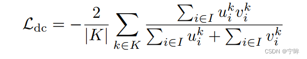
- μ是网络的softmax输出
- v是分割标签的one-hot编码
import torch
import torch.nn as nn
import torch.nn.functional as F
from einops import rearrange# 二分割的dice loss其实可以写的更简单,但我懒得简化了
class Loss(nn.Module):def __init__(self, n_classes, alpha=0.5):"dice_loss_plus_cetr_weighted"super(Loss, self).__init__()self.n_classes = n_classesself.alpha = alphadef forward(self, input, target):smooth = 0.01input1 = F.softmax(input, dim=1)target1 = F.one_hot(target,self.n_classes)input1 = rearrange(input1,'b n h w s -> b n (h w s)')target1 = rearrange(target1,'b h w s n -> b n (h w s)')# 只取前景input1 = input1[:, 1:, :]target1 = target1[:, 1:, :].float()# dice lossinter = torch.sum(input1 * target1)union = torch.sum(input1) + torch.sum(target1) + smoothdice = 2.0 * inter / union# 交叉熵loss = F.cross_entropy(input,target)total_loss = (1 - self.alpha) * loss + (1 - dice) * self.alphareturn total_lossif __name__ == '__main__':torch.manual_seed(3)device = torch.device('cuda' if torch.cuda.is_available() else 'cpu')losser = Loss(n_classes=2).to(device)x = torch.randn((2, 2, 16, 16, 16)).to(device)y = torch.randint(0, 2, (2, 16, 16, 16)).to(device)print(losser(x, y))
训练框架
import os
import torch
import argparse
import torch.optim as optim
from tqdm import tqdm
from torch.utils.data import DataLoader
from torchvision import transforms
from networks.vnet import VNet
from loss import Loss
from dataloaders.la_heart import LAHeart, RandomCrop, CenterCrop, RandomRotFlip, ToTensordef cal_dice(output, target, eps=1e-3):output = torch.argmax(output,dim=1)inter = torch.sum(output * target) + epsunion = torch.sum(output) + torch.sum(target) + eps * 2dice = 2 * inter / unionreturn dicedef train_loop(model, optimizer, criterion, train_loader, device):model.train()running_loss = 0pbar = tqdm(train_loader)dice_train = 0for sampled_batch in pbar:volume_batch, label_batch = sampled_batch['image'], sampled_batch['label']volume_batch, label_batch = volume_batch.to(device), label_batch.to(device)# print(volume_batch.shape,label_batch.shape)outputs = model(volume_batch)# print(outputs.shape)loss = criterion(outputs, label_batch)dice = cal_dice(outputs, label_batch)dice_train += dice.item()pbar.set_postfix(loss="{:.3f}".format(loss.item()), dice="{:.3f}".format(dice.item()))running_loss += loss.item()optimizer.zero_grad()loss.backward()optimizer.step()loss = running_loss / len(train_loader)dice = dice_train / len(train_loader)return {'loss': loss, 'dice': dice}def eval_loop(model, criterion, valid_loader, device):model.eval()running_loss = 0pbar = tqdm(valid_loader)dice_valid = 0with torch.no_grad():for sampled_batch in pbar:volume_batch, label_batch = sampled_batch['image'], sampled_batch['label']volume_batch, label_batch = volume_batch.to(device), label_batch.to(device)outputs = model(volume_batch)loss = criterion(outputs, label_batch)dice = cal_dice(outputs, label_batch)running_loss += loss.item()dice_valid += dice.item()pbar.set_postfix(loss="{:.3f}".format(loss.item()), dice="{:.3f}".format(dice.item()))loss = running_loss / len(valid_loader)dice = dice_valid / len(valid_loader)return {'loss': loss, 'dice': dice}def train(args, model, optimizer, criterion, train_loader, valid_loader, epochs,device, train_log, loss_min=999.0):for e in range(epochs):# train for epochtrain_metrics = train_loop(model, optimizer, criterion, train_loader, device)valid_metrics = eval_loop(model, criterion, valid_loader, device)# eval for epochinfo1 = "Epoch:[{}/{}] train_loss: {:.3f} valid_loss: {:.3f}".format(e + 1, epochs, train_metrics["loss"],valid_metrics['loss'])info2 = "train_dice: {:.3f} valid_dice: {:.3f}".format(train_metrics['dice'], valid_metrics['dice'])print(info1 + '\n' + info2)with open(train_log, 'a') as f:f.write(info1 + '\n' + info2 + '\n')if valid_metrics['loss'] < loss_min:loss_min = valid_metrics['loss']torch.save(model.state_dict(), args.save_path)print("Finished Training!")def main(args):torch.manual_seed(args.seed)  # 为CPU设置种子用于生成随机数,以使得结果是确定的torch.cuda.manual_seed_all(args.seed)  # 为所有的GPU设置种子,以使得结果是确定的torch.backends.cudnn.deterministic = Truetorch.backends.cudnn.benchmark = Trueos.environ['CUDA_VISIBLE_DEVICES'] = '0'device = torch.device('cuda' if torch.cuda.is_available() else 'cpu')# data infodb_train = LAHeart(base_dir=args.train_path,split='train',transform=transforms.Compose([RandomRotFlip(),RandomCrop(args.patch_size),ToTensor(),]))db_test = LAHeart(base_dir=args.train_path,split='test',transform=transforms.Compose([CenterCrop(args.patch_size),ToTensor()]))print('Using {} images for training, {} images for testing.'.format(len(db_train), len(db_test)))trainloader = DataLoader(db_train, batch_size=args.batch_size, shuffle=True, num_workers=4, pin_memory=True,drop_last=True)testloader = DataLoader(db_test, batch_size=1, num_workers=4, pin_memory=True)model = VNet(n_channels=1,n_classes=args.num_classes, normalization='batchnorm', has_dropout=True).to(device)criterion = Loss(n_classes=args.num_classes).to(device)optimizer = optim.SGD(model.parameters(), momentum=0.9, lr=args.lr, weight_decay=1e-4)# 加载训练模型if os.path.exists(args.weight_path):weight_dict = torch.load(args.weight_path, map_location=device)model.load_state_dict(weight_dict)print('Successfully loading checkpoint.')train(args, model, optimizer, criterion, trainloader, testloader, args.epochs, device, train_log=args.train_log)if __name__ == '__main__':parser = argparse.ArgumentParser()parser.add_argument('--num_classes', type=int, default=2)parser.add_argument('--seed', type=int, default=21)parser.add_argument('--epochs', type=int, default=160)parser.add_argument('--batch_size', type=int, default=4)parser.add_argument('--lr', type=float, default=0.01)parser.add_argument('--patch_size', type=float, default=(112, 112, 80))parser.add_argument('--train_path', type=str, default='/***/LASet/data')parser.add_argument('--train_log', type=str, default='results/VNet_sup.txt')parser.add_argument('--weight_path', type=str, default='results/VNet_sup.pth')  # 加载parser.add_argument('--save_path', type=str, default='results/VNet_sup.pth')  # 保存args = parser.parse_args()main(args)
实验结果
训练


Epoch:[1/160] train_loss: 0.670 valid_loss: 0.559
train_dice: 0.337 valid_dice: 0.192
Epoch:[2/160] train_loss: 0.522 valid_loss: 0.567
train_dice: 0.317 valid_dice: 0.143
......
Epoch:[160/160] train_loss: 0.066 valid_loss: 0.090
train_dice: 0.939 valid_dice: 0.924
任务比较简单,因此收敛的很快。
注意,这里的dice是测试集中心裁剪的dice,真实指标需要使用滑动窗口进行推理,代码我放在了
inference.py
推理
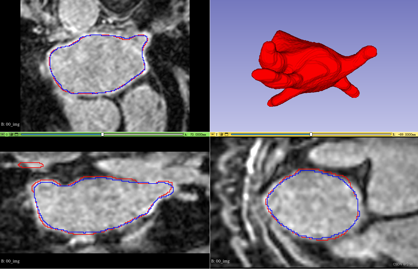
图中,红色的是标签轮廓,蓝色的是 VNet 网络预测结果的轮廓。
import math
import torch
import torch.nn.functional as F
import numpy as np
import h5py
import nibabel as nib
from medpy import metric
from networks.vnet import VNetdef calculate_metric_percase(pred, gt):dice = metric.binary.dc(pred, gt)jc = metric.binary.jc(pred, gt)hd = metric.binary.hd95(pred, gt)asd = metric.binary.asd(pred, gt)return dice, jc, hd, asddef test_single_case(net, image, stride_xy, stride_z, patch_size, num_classes=1):w, h, d = image.shape# if the size of image is less than patch_size, then padding itadd_pad = Falseif w < patch_size[0]:w_pad = patch_size[0]-wadd_pad = Trueelse:w_pad = 0if h < patch_size[1]:h_pad = patch_size[1]-hadd_pad = Trueelse:h_pad = 0if d < patch_size[2]:d_pad = patch_size[2]-dadd_pad = Trueelse:d_pad = 0wl_pad, wr_pad = w_pad//2,w_pad-w_pad//2hl_pad, hr_pad = h_pad//2,h_pad-h_pad//2dl_pad, dr_pad = d_pad//2,d_pad-d_pad//2if add_pad:image = np.pad(image, [(wl_pad,wr_pad),(hl_pad,hr_pad), (dl_pad, dr_pad)], mode='constant', constant_values=0)ww,hh,dd = image.shapesx = math.ceil((ww - patch_size[0]) / stride_xy) + 1sy = math.ceil((hh - patch_size[1]) / stride_xy) + 1sz = math.ceil((dd - patch_size[2]) / stride_z) + 1# print("{}, {}, {}".format(sx, sy, sz))score_map = np.zeros((num_classes, ) + image.shape).astype(np.float32)cnt = np.zeros(image.shape).astype(np.float32)for x in range(0, sx):xs = min(stride_xy*x, ww-patch_size[0])for y in range(0, sy):ys = min(stride_xy * y,hh-patch_size[1])for z in range(0, sz):zs = min(stride_z * z, dd-patch_size[2])test_patch = image[xs:xs+patch_size[0], ys:ys+patch_size[1], zs:zs+patch_size[2]]test_patch = np.expand_dims(np.expand_dims(test_patch,axis=0),axis=0).astype(np.float32)test_patch = torch.from_numpy(test_patch).cuda()y1 = net(test_patch)y = F.softmax(y1, dim=1)y = y.cpu().data.numpy()y = y[0,:,:,:,:]score_map[:, xs:xs+patch_size[0], ys:ys+patch_size[1], zs:zs+patch_size[2]] \= score_map[:, xs:xs+patch_size[0], ys:ys+patch_size[1], zs:zs+patch_size[2]] + ycnt[xs:xs+patch_size[0], ys:ys+patch_size[1], zs:zs+patch_size[2]] \= cnt[xs:xs+patch_size[0], ys:ys+patch_size[1], zs:zs+patch_size[2]] + 1score_map = score_map/np.expand_dims(cnt,axis=0)label_map = np.argmax(score_map, axis = 0)if add_pad:label_map = label_map[wl_pad:wl_pad+w,hl_pad:hl_pad+h,dl_pad:dl_pad+d]score_map = score_map[:,wl_pad:wl_pad+w,hl_pad:hl_pad+h,dl_pad:dl_pad+d]return label_map, score_mapdef test_all_case(net, image_list, num_classes=2, patch_size=(112, 112, 80), stride_xy=18, stride_z=4, save_result=True, test_save_path=None, preproc_fn=None):total_metric = 0.0for ith,image_path in enumerate(image_list):h5f = h5py.File(image_path, 'r')image = h5f['image'][:]label = h5f['label'][:]if preproc_fn is not None:image = preproc_fn(image)prediction, score_map = test_single_case(net, image, stride_xy, stride_z, patch_size, num_classes=num_classes)if np.sum(prediction)==0:single_metric = (0,0,0,0)else:single_metric = calculate_metric_percase(prediction, label[:])print('%02d,\t%.5f, %.5f, %.5f, %.5f' % (ith, single_metric[0], single_metric[1], single_metric[2], single_metric[3]))total_metric += np.asarray(single_metric)if save_result:nib.save(nib.Nifti1Image(prediction.astype(np.float32), np.eye(4)), test_save_path + "%02d_pred.nii.gz"%(ith))nib.save(nib.Nifti1Image(image[:].astype(np.float32), np.eye(4)), test_save_path + "%02d_img.nii.gz"%(ith))nib.save(nib.Nifti1Image(label[:].astype(np.float32), np.eye(4)), test_save_path + "%02d_gt.nii.gz"%(ith))avg_metric = total_metric / len(image_list)print('average metric is {}'.format(avg_metric))return avg_metricif __name__ == '__main__':data_path = '/***/data_set/LASet/data/'test_save_path = 'predictions/'save_mode_path = 'results/VNet.pth'net = VNet(n_channels=1,n_classes=2, normalization='batchnorm').cuda()net.load_state_dict(torch.load(save_mode_path))print("init weight from {}".format(save_mode_path))net.eval()with open(data_path + '/../test.list', 'r') as f:image_list = f.readlines()image_list = [data_path +item.replace('\n', '')+"/mri_norm2.h5" for item in image_list]# 滑动窗口法avg_metric = test_all_case(net, image_list, num_classes=2,patch_size=(112, 112, 80), stride_xy=18, stride_z=4,save_result=True,test_save_path=test_save_path)
init weight from results/VNet.pth
00,     0.90632, 0.82868, 6.40312, 1.27997
01,     0.89492, 0.80982, 6.48074, 1.14056
......
30,     0.94105, 0.88866, 3.16228, 1.03454
average metric is [0.91669405 0.84675762 5.33117527 1.42431875]
这个数据集也比较简单,常用来做半监督分割,以后也会更新一些半监督学习的内容。码字不易,有用的话还请点个赞。
项目github地址:LASeg: 2018 Left Atrium Segmentation (MRI)
代码参考 https://github.com/yulequan/UA-MT 以及 https://github.com/ycwu1997/MC-Net