实验9 分类问题

1. 实验目的

①掌握逻辑回归的基本原理，实现分类器，完成多分类任务；
②掌握逻辑回归中的平方损失函数、交叉熵损失函数以及平均交叉熵损失函数。

2. 实验内容

①能够使用TensorFlow计算Sigmoid函数、准确率、交叉熵损失函数等，并在此基础上建立逻辑回归模型，完成分类任务；
②能够使用MatPlotlib绘制分类图。

3. 实验过程

题目一：

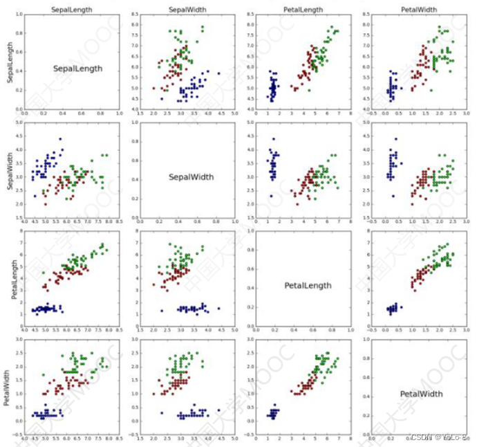
观察6.5.3小节中给出的鸢尾花数据集可视化结果(如图1所示)，编写代码实现下述功能：(15分)
在这里插入图片描述

图1 鸢尾花数据集

要求：
⑴选择恰当的属性或属性组合，训练逻辑回归模型，区分山鸢尾和维吉尼亚鸢尾，并测试模型性能，以可视化的形式展现训练和测试的过程及结果。
⑵比较选择不同属性或属性组合时的学习率、迭代次数，以及在训练集和测试集上的交叉熵损失和准确率，以表格或合适的图表形式展示。
⑶分析和总结：
区分山鸢尾和维吉尼亚鸢尾，至少需要几种属性？说明选择某种属性或属性组合的依据；通过以上结果，可以得到什么结论，或对你有什么启发。
① 代码

import math
import randomimport tensorflow as tf
import pandas as pd
import numpy as np
import matplotlib as mpl
import matplotlib.pyplot as plt#下载鸢尾花训练数据集和测试数据集
TRAIN_URL = "http://download.tensorflow.org/data/iris_training.csv"
train_path = tf.keras.utils.get_file(TRAIN_URL.split('/')[-1],TRAIN_URL)TEST_URL = "http://download.tensorflow.org/data/iris_test.csv"
test_path = tf.keras.utils.get_file(TEST_URL.split("/")[-1],TEST_URL)#读取数据集并转换为numpy数组
df_iris_train = pd.read_csv(train_path, header=0)
df_iris_test = pd.read_csv(test_path,header=0)
iris_train = np.array(df_iris_train)
iris_test = np.array(df_iris_test)#提取分量,花萼的长度和宽度来训练模型
train_x = iris_train[:,(0,1)]
train_y = iris_train[:,4]
test_x = iris_test[:,(0,1)]
test_y = iris_test[:,4]#有三种鸢尾花的品种，采取以下方法提取出山鸢尾和维吉尼亚鸢尾
x_train = train_x[train_y != 1]
y_train = train_y[train_y != 1]
x_test = test_x[test_y != 1]
y_test = test_y[test_y != 1]#将维吉尼亚鸢尾的值赋为1
y_train[y_train == 2] = 1
y_test[y_test == 2] = 1num_train = len(x_train)
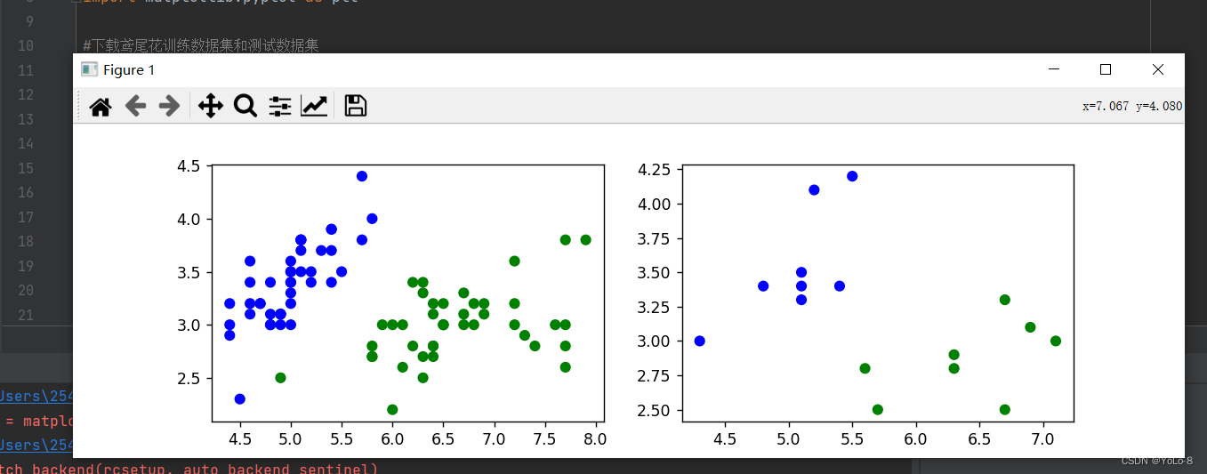
num_test = len(x_test)plt.figure(figsize=(10,3))
cm_pt = mpl.colors.ListedColormap(["blue","green"])plt.subplot(121)
plt.scatter(x_train[:,0],x_train[:,1],c = y_train,cmap=cm_pt)plt.subplot(122)
plt.scatter(x_test[:,0],x_test[:,1],c = y_test,cmap=cm_pt)
plt.show()#按列中心化
x_train = x_train - np.mean(x_train,axis=0)
x_test = x_test - np.mean(x_test,axis=0)"""
plt.figure(figsize=(10,3))
cm_pt = mpl.colors.ListedColormap(["blue","green"])plt.subplot(121)
plt.scatter(x_train[:,0],x_train[:,1],c = y_train,cmap=cm_pt)plt.subplot(122)
plt.scatter(x_test[:,0],x_test[:,1],c = y_test,cmap=cm_pt)
plt.show()
"""x0_train = np.ones(num_train).reshape(-1,1)
X_train = tf.cast(tf.concat((x0_train,x_train),axis=1),tf.float32)
Y_train = tf.cast(y_train.reshape(-1,1),tf.float32)x0_test = np.ones(num_test).reshape(-1,1)
X_test = tf.cast(tf.concat((x0_test,x_test),axis=1),tf.float32)
Y_test = tf.cast(y_test.reshape(-1,1),tf.float32)#设置超参数
learn_rate = 0.2
iter = 200
display_step = 50np,random.seed(612)
W = tf.Variable(np.random.randn(3,1),dtype=tf.float32)ce_train = []
ce_test = []
acc_train = []
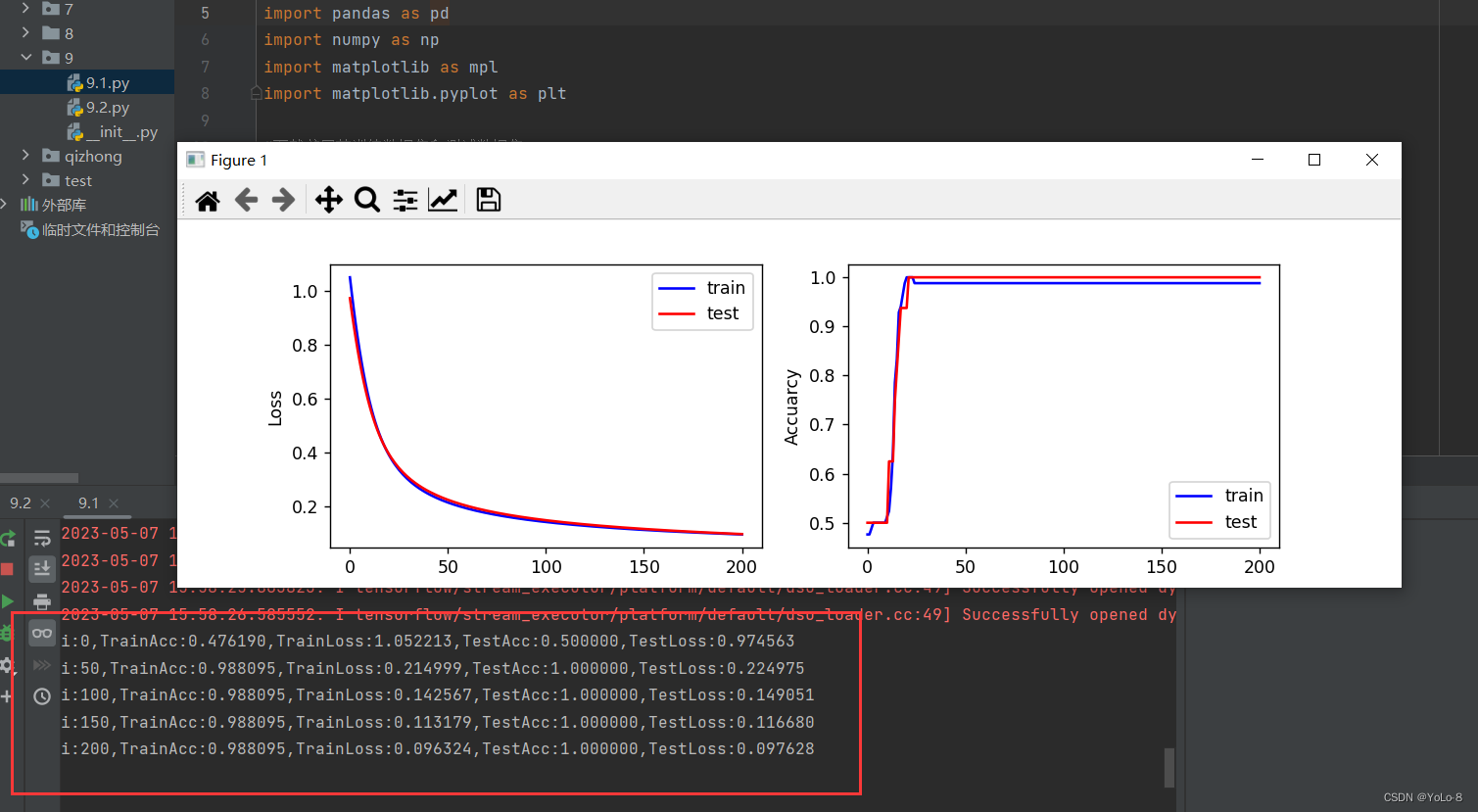
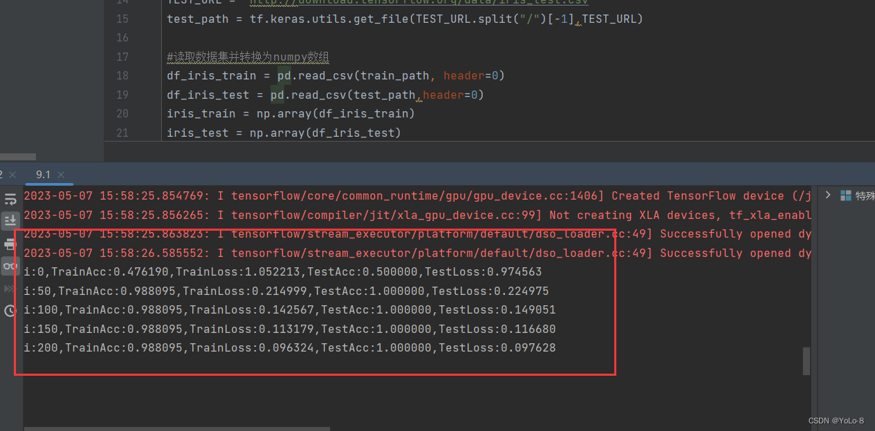
acc_test = []for i in range(0,iter + 1):with tf.GradientTape() as tape:PRED_train = 1 / (1 + tf.exp(-tf.matmul(X_train,W)))Loss_train = -tf.reduce_mean(Y_train * tf.math.log(PRED_train) + (1 - Y_train) * tf.math.log(1 - PRED_train))PRED_test = 1 / (1 + tf.exp(- tf.matmul(X_test,W)))Loss_test = -tf.reduce_mean(Y_test * tf.math.log(PRED_test) + (1 - Y_test) * tf.math.log(1 - PRED_test))accuracy_train = tf.reduce_mean(tf.cast(tf.equal(tf.where(PRED_train.numpy() < 0.5,0.,1.),Y_train),tf.float32))accuracy_test = tf.reduce_mean(tf.cast(tf.equal(tf.where(PRED_test.numpy() < 0.5,0.,1.),Y_test),tf.float32))ce_train.append(Loss_train)acc_train.append(accuracy_train)ce_test.append(Loss_test)acc_test.append(accuracy_test)dL_dW = tape.gradient(Loss_train,W)W.assign_sub(learn_rate * dL_dW)if i % display_step == 0:print("i:%d,TrainAcc:%f,TrainLoss:%f,TestAcc:%f,TestLoss:%f"%(i,accuracy_train,Loss_train,accuracy_test,Loss_test))plt.figure(figsize=(10,3))plt.subplot(121)
plt.plot(ce_train,color="b",label = "train")
plt.plot(ce_test,color="r",label = "test")
plt.ylabel("Loss")
plt.legend()plt.subplot(122)
plt.plot(acc_train,color="b",label = "train")
plt.plot(acc_test,color="r",label = "test")
plt.ylabel("Accuarcy")
plt.legend()
plt.show()

② 结果记录
在这里插入图片描述

③ 实验总结

在这里插入图片描述

题目二：

在Iris数据集中，分别选择2种、3种和4种属性，编写程序，区分三种鸢尾花。记录和分析实验结果，并给出总结。(20分)
⑴确定属性选择方案。
⑵编写代码建立、训练并测试模型。
⑶参考11.6小节例程，对分类结果进行可视化。
⑷分析结果：
比较选择不同属性组合时的学习率、迭代次数、以及在训练集和测试集上的交叉熵损失和准确率，以表格或合适的图表形式展示。
(3)总结：
通过以上分析和实验结果，对你有什么启发。

① 代码

import tensorflow as tf
import numpy as np
import pandas as pd
import matplotlib as mpl
import matplotlib.pyplot as pltTRAIN_URL = "http://download.tensorflow.org/data/iris_training.csv"
train_path = tf.keras.utils.get_file(TRAIN_URL.split("/")[-1], TRAIN_URL)df_iris_train = pd.read_csv(train_path,header=0)
iris_train = np.array(df_iris_train)
x_train = iris_train[:,2:4]
y_train = iris_train[:,4]
num_train = len(x_train)x0_train = np.ones(num_train).reshape(-1,1)
X_train = tf.cast(tf.concat([x0_train,x_train],axis=1),tf.float32)
Y_train = tf.one_hot(tf.constant(y_train,dtype=tf.int32),3)learn_rate = 0.2
iter = 700
display = 100np.random.seed(612)
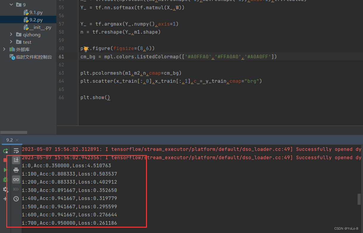
W = tf.Variable(np.random.randn(3,3),dtype=tf.float32)acc = []
cce = []for i in range(iter + 1):with tf.GradientTape() as tape:PRED_train = tf.nn.softmax(tf.matmul(X_train,W))Loss_train = -tf.reduce_sum(Y_train * tf.math.log(PRED_train)) / num_trainaccuracy_train = tf.reduce_mean(tf.cast(tf.equal(tf.argmax(PRED_train.numpy(),axis=1),y_train),tf.float32))acc.append(accuracy_train)cce.append(Loss_train)dL_dW = tape.gradient(Loss_train,W)W.assign_sub(learn_rate * dL_dW)if i % display == 0:print("i:%d,Acc:%f,Loss:%f"%(i,accuracy_train,Loss_train))M = 500
x1_min,x2_min = x_train.min(axis = 0)
x1_max,x2_max = x_train.max(axis = 0)
t1 = np.linspace(x1_min,x1_max,M)
t2 = np.linspace(x2_min,x2_max,M)
m1,m2 = np.meshgrid(t1,t2)m0 = np.ones(M * M)
X_ = tf.cast(np.stack((m0,m1.reshape(-1),m2.reshape(-1)),axis=1),tf.float32)
Y_ = tf.nn.softmax(tf.matmul(X_,W))Y_ = tf.argmax(Y_.numpy(),axis=1)
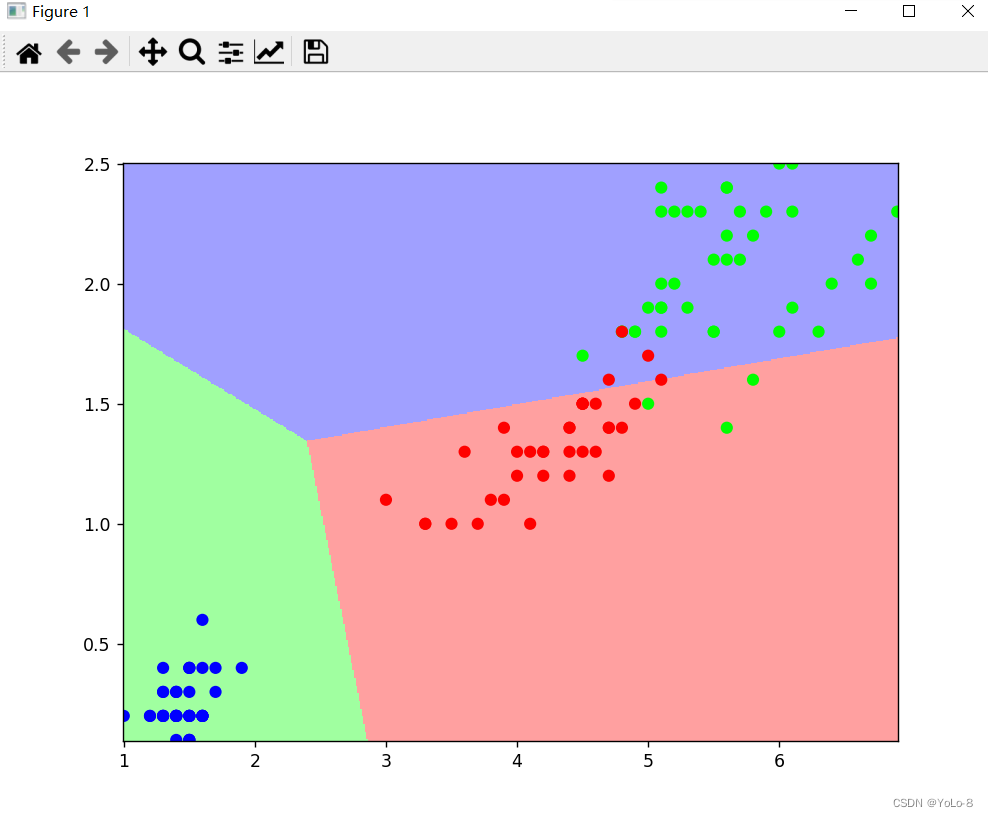
n = tf.reshape(Y_,m1.shape)plt.figure(figsize=(8,6))
cm_bg = mpl.colors.ListedColormap(['#A0FFA0','#FFA0A0','#A0A0FF'])plt.pcolormesh(m1,m2,n,cmap=cm_bg)
plt.scatter(x_train[:,0],x_train[:,1],c = y_train,cmap="brg")plt.show()

② 结果记录
在这里插入图片描述

③ 实验总结
在这里插入图片描述

4. 实验小结&讨论题

①实现分类问题的一般步骤是什么？实现二分类和多分类问题时有什么不同之处？哪些因素会对分类结果产生影响?
答：1.问题的提出2.神经网络模型的搭建和训3.结果展示。
多分类：
每个样本只能有一个标签，比如ImageNet图像分类任务，或者MNIST手写数字识别数据集，每张图片只能有一个固定的标签。
对单个样本，假设真实分布为，网络输出分布为，总的类别数为，则在这种情况下，交叉熵损失函数的计算方法如下所示，我们可以看出，实际上也就是计算了标签类别为1的交叉熵的值，使得对应的信息量越来越小，相应的概率也就越来越大了。
二分类：
对于二分类，既可以选择多分类的方式，也可以选择多标签分类的方式进行计算，结果差别也不会太大
②将数据集划分为训练集和测试集时，应该注意哪些问题？改变训练集和测试集所占比例，对分类结果会有什么影响？
答：同样的迭代次数，和学习率下，随着训练集的比例逐渐变大，训练集交叉熵损失大致变小准确率变高的趋势，测试集交叉熵损失大致变大准确率变高的趋势。

③当数据集中存在缺失值时，有哪些处理的方法？查阅资料并结合自己的思考，说明不同处理方法的特点和对分类结果的影响。
答：
（1）删除，直接去除含有缺失值的记录，适用于数据量较大（记录较多）且缺失比较较小的情形，去掉后对总体影响不大。
（2）常量填充，变量的含义、获取方式、计算逻辑，以便知道该变量为什么会出现缺失值、缺失值代表什么含义。
（3）插值填充，采用某种插入模式进行填充，比如取缺失值前后值的均值进行填充。
（4）KNN填充
（5）随机森林填充，随机森林算法填充的思想和knn填充是类似的，即利用已有数据拟合模型，对缺失变量进行预测。