Introduction

• 作者提出 Optimal brain damage (OBD) 的改进 Optimal brain surgeon (OBS) 用于模型剪枝

Method

Optimal brain surgeon (OBS)

• 类似于 Optimal brain damage (OBD)，OBS 也将 $\delta E$ 用泰勒公式展开
  其中，$E$ 为损失函数，$w$ 为权重向量，$H={\partial }^{2}E/\partial w^2$ 为 Hessian matrix. 类似于 OBD，为了简化上式，作者假设剪枝前模型权重已位于局部最小点从而省略第一项，假设目标函数近似二次函数从而省略第三项，但需要注意的是，不同于 OBD，这里作者并没有使用 “diagonal” approximation，不假设 $H$ 为对角矩阵。这样上式就简化为了
  $$\delta E=\frac{1}{2}\delta w^T\cdot H\cdot \delta w$$
• 在剪枝过程中，对 $w_q$ 进行剪枝可以表示为 $\delta w_q+w_q=0$，也可以被表示为
  其中，$e_q$ 为对应 (scalar) weight $w_q$ 的单位向量。这样剪枝过程可以被表示为求解如下最优化问题：
  求解完成后对 $w_q$ 进行剪枝即可。为了解上式，可以将其写为拉格朗日展式：
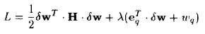  对其求解可以得到 optimal weight change 和 resulting change in error 分别为
  
• Optimal Brain Surgeon procedure. 可以看到，OBS 其实是 OBD 的推广，首先 OBS 不假设 $H$ 为对角矩阵；其次在进行剪枝后，OBS 会对所有权重参数进行更新，从而对被剪枝的权重进行补偿，使得损失函数在剪枝后尽可能更小
  

Computing the inverse Hessian

• 现在唯一的问题就是如何高效计算 $H^{-1}$，为此作者提出了 outer-product approximation

---

计算 $H$

• 现在考虑非线性网络 $F$
  其中，$\mathbf{in}$ 为输入向量，$\mathbf{w}$ 为权重，$\mathbf{o}$ 为输出向量。训练集上的均方误差可以表示为
  由此可以计算出 $\mathbf{w}$ 的一阶导
  注意上式中的 $\frac{\partial F(\mathbf{w},{\mathbf{in}}^{[k]})}{\partial \mathbf{w}}({\mathbf{t}}^{[k]}-{\mathbf{o}}^{[k]})$ 为向量逐元素乘。进一步可以推出二阶导 / Hessian 为
  
• 下面对上式做进一步简化。假设模型已经达到了误差局部极小点，此时可以 ${\mathbf{t}}^{[k]}-{\mathbf{o}}^{[k]}\approx 0$ 可以忽略 (Even late in pruning, when this error is not small for a single pattern, this approximation can be justified, explained in the nest section)，由此可得
  令
  则得到了 Hessian matrix 的 outer-product approximation
  其中，$P$ 为训练集样本数，${\mathbf{X}}^{[k]}$ 为第 $k$ 个样本的 $n$-dimensional data vector of derivatives. 假如网络有多个输出，则 $\mathbf{X}$ 为
  Hessian matrix 为
  
• 考虑模型只有单一输出的情况，我们可以遍历训练集，迭代地计算 $H$
  其中，$H_0=\alpha I$，$H_P=H$

---

计算 $H^{-1}$

• 根据 Woodbury identity 可知，
  将其代入 $H$ 的迭代式可知，
  其中，$H_0^{-1}={\alpha }^{-1}I$，$H_P^{-1}=H^{-1}$，$\alpha$ ($10^{-8}\le \alpha \le 10^{-4}$) 为 a small constant needed to make $H_0^{-1}$ meaningful.
• 实际上，上述迭代求解出的 $H_P^{-1}$ 为 $(H+\alpha I)$ 的逆。原来的拉格朗日展式为
  如果将 $H$ 替换为 $(H+\alpha I)$，则相当于是加上了正则项 $\alpha \Vert \delta \mathbf{w}{\Vert }^2$，可以避免剪枝后权重向量值更新过大，同时也保证了将 $\delta E$ 用泰勒公式展开时忽略高次项的合理性

The $(\mathbf{t}-\mathbf{o})\to 0$ Approximation

• Computational view. $\mathbf{H}$ 在剪枝前通常是不可逆的，$(\mathbf{t}-\mathbf{o})\to 0$ 的近似可以保证 ${\mathbf{H}}^{-1}$ 的计算是有良好定义的. In Statistics the approximation is the basis of Fisher’s method of scoring and its goal is to replace tlie true Hessian with its expected value and hence guarantee that $\mathbf{H}$ is positive definite.
• Functional justifications. (这里没看太明白) Consider a high capacity network trained to small training error. We can consider the network structure as involving both signal and noise. As we prune, we hope to eliminate those weights that lead to “overfitting.” i.e., learning the noise. If our pruning method did not employ the $(\mathbf{t}-\mathbf{o})\to 0$ approximation, every pruning step (Eqs. 9 and 8) would inject the noise back into the system, by penalizing for noise terms. A different way to think of the approximation is the following. After some pruning by OBS we have
  reached a new weight vector that is a local minimum of the error. Even if this error is not negligible, we want to stay as close to that value of the error as we can. Thus we imagine a new effective teaching signal ${\mathbf{t}}^{\ast }$, that would keep the network near this new error minimum. It is then $({\mathbf{t}}^{\ast }-\mathbf{o})$ that we in effect set to zero when using Eq. 11 instead of Eq. 10.

References

• Hassibi, Babak, David G. Stork, and Gregory J. Wolff. “Optimal brain surgeon and general network pruning.” IEEE international conference on neural networks. IEEE, 1993.