色带通用型号表_Excel表中基于日期的色带

色带通用型号表

When you create a named table in Excel, you can colour the alternating rows with one of the built-in Table Styles. But how could you colour alternating groups of information, such as dates? This example shows show to create colour bands, based on dates, so it's easy to see where each day's data begins and ends.

在Excel中创建命名表时，可以使用内置的表样式之一为交替的行着色。但是，如何为交替的信息组(例如日期)着色？此示例显示了根据日期创建色带的显示，因此很容易看到每天数据的开始和结束位置。

Excel中的色带 (Colour Bands in Excel)

In the steps shown below, you'll see how to use Excel conditional formatting to create colour bands, based on the data in one column..

在下面显示的步骤中，您将看到如何基于一列中的数据使用Excel条件格式来创建色带。

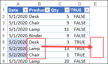
In this example, the sales rows for the dates are in alternating colours - blue and no fill. This technique was adapted from Chip Pearson's site.

在此示例中，日期的销售行以交替的颜色显示-蓝色且没有填充。该技术改编自Chip Pearson的站点。

添加新列 (Add a New Column)

First, we need to add a new column to the table, where a formula will check the date, and compare it with the date in the previous row.

首先，我们需要在表中添加一个新列，公式将在该列中检查日期，并将其与上一行中的日期进行比较。

In cell D1, type a heading for a new column - TRUE
在单元格D1中，输入新列的标题-TRUE
In cell D2, enter this formula, to compare the dates:
在单元格D2中，输入以下公式，以比较日期：
=IF(A1=A2,D1,NOT(D1))
= IF(A1 = A2，D1，NOT(D1))
Press Enter, and the formula automatically fills down to the end of the table, with a result of TRUE or FALSE in each row.
按Enter键，公式将自动填充到表格末尾，每行结果为TRUE或FALSE。

Colour Bands in Excel Table Based on Dates

公式如何运作 (How the Formula Works)

The formula in cell D2 compares the date in column A, to the date in the cell above that

D2单元格中的公式将A列中的日期与该日期上方的单元格中的日期进行比较

=IF(A1=A2,D1,NOT(D1))

= IF( A1 = A2 ，D1，NOT(D1))

If the dates are the same, the result is the value from column D, in the previous row

如果日期相同，则结果为上一行中D列的值

=IF(A1=A2,D1,NOT(D1))

= IF(A1 = A2， D1 ，NOT(D1))

If the dates are different, the result is the opposite of the value in the row above, because the Excel NOT function reverses TRUE and FALSE.

如果日期不同，则结果与上一行中的值相反，因为Excel NOT函数将TRUE和FALSE取反。

=IF(A1=A2,D1,NOT(D1))

= IF(A1 = A2，D1， NOT(D1) )

In cell D2, the result is FALSE (the opposite of the TRUE in cell D1), because the date in cell A1 is not equal to the "Date" heading in cell A1.

在单元格D2中，结果为FALSE(与单元格D1中的TRUE相反)，因为单元格A1中的日期不等于单元格A1中的“日期”标题。

NOTE: You could use either TRUE or FALSE as the heading in column D

注意：您可以使用TRUE或FALSE作为D列的标题

桌上型Opton (Table Style Optons)

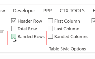
Before you add the conditional formatting, turn off banded rows in your Excel table, if that feature is active.

在添加条件格式之前，如果该功能处于活动状态，请关闭Excel表中的带状行。

Select a cell in the table
在表格中选择一个单元格
On the Excel Ribbon, click the Table Design tab
在Excel功能区上，单击“表设计”选项卡
In the Table Style Options group, remove the check mark for Banded Rows.
在“表格样式选项”组中，删除“带状行”的复选标记。

添加条件格式 (Add Conditional Formatting)

Then, follow these steps to add the conditional formatting that creates colour bands:

然后，请按照下列步骤添加创建色带的条件格式：

Starting from row 2, select all the data cells in the table
从第2行开始，选择表中的所有数据单元格
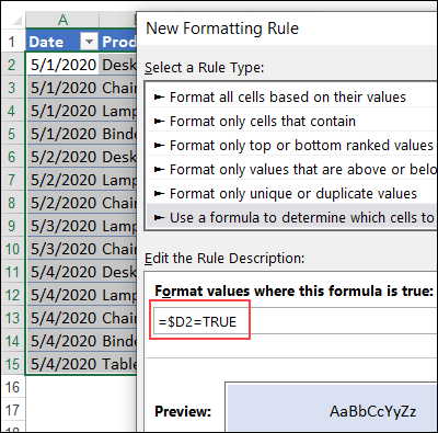
On the Home tab, click Conditional Formatting, New Rule
在“开始”选项卡上，单击“条件格式，新规则”
Click on "Use a formula to determine which cells to format"
单击“使用公式来确定要格式化的单元格”
In the formula box, type this formula, referring to the active data cell:
在公式框中，键入以下公式，以引用活动数据单元格：
=$D2=TRUE
= $ D2 = TRUE
Click the Format button, and choose a fill colour for the rows that have TRUE in column D
单击格式按钮，然后为D列中为TRUE的行选择填充颜色
Click OK, twice, to apply the formatting
单击确定两次，以应用格式
(Optional) Hide the TRUE/FALSE column, to tidy up the worksheet.
(可选)隐藏TRUE / FALSE列，以整理工作表。

绝对参考 (Absolute Reference)

In the conditional formatting rule, =$D2=TRUE, we use an absolute reference to column D ($D), instead of a relative reference (D).

在条件格式化规则= $ D2 = TRUE中 ，我们使用对列D( $ D )的绝对引用，而不是相对引用( D )。

With an absolute reference, all the columns will refer to the value in column D
对于绝对引用，所有列均将引用D列中的值
With a relative reference, the formula would adjust in each column, and each cell would check its own value, instead of the cell in column D.
使用相对引用，该公式将在每列中进行调整，并且每个单元格将检查其自己的值，而不是D列中的单元格。

For example, the conditional formatting in column B would look for TRUE in column E, instead of column D. Column E is empty, so there's no colour applied in column B.

例如，B列中的条件格式将在E列而不是D列中查找TRUE。E列为空，因此B列中没有应用颜色。