工业场景下的滚珠丝杠传动表面缺陷分割检测系统在我们前面的博文中已经有了相关的开发实践了，感兴趣的话可以自行阅读即可：

《助力工业生产质检，基于轻量级yolov5-seg开发构建工业场景下滚珠丝杠传动表面缺陷分割检测系统》

前文主要是以seg系列最为轻量级的模型作为基准开发模型来进行模型的开发构建的，本文的主要目的是想要应用开发seg全系列不同参数量级的模型来综合对比不同量级参数模型的性能结果，首先看下实例效果：

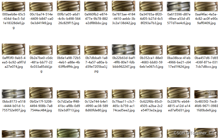
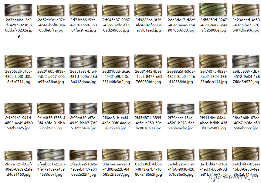
简单看下数据集：

这里我直接使用的是官方v7.0分支的代码，项目地址在这里，如下所示：

如果不会使用可以参考我的教程：

《基于yolov5-v7.0开发实践实例分割模型超详细教程》

非常详细的操作实践教程，这里就不再赘述了。

训练数据配置文件如下所示：

#Dataset
path: ./dataset
train: images/train 
val: images/train  
test:  images/train # Classes
names:0: Pitting

【n系列模型】

# YOLOv5 🚀 by Ultralytics, GPL-3.0 license# Parameters
nc: 1  # number of classes
depth_multiple: 0.33  # model depth multiple
width_multiple: 0.25  # layer channel multiple
anchors:- [10,13, 16,30, 33,23]  # P3/8- [30,61, 62,45, 59,119]  # P4/16- [116,90, 156,198, 373,326]  # P5/32# YOLOv5 v6.0 backbone
backbone:# [from, number, module, args][[-1, 1, Conv, [64, 6, 2, 2]],  # 0-P1/2[-1, 1, Conv, [128, 3, 2]],  # 1-P2/4[-1, 3, C3, [128]],[-1, 1, Conv, [256, 3, 2]],  # 3-P3/8[-1, 6, C3, [256]],[-1, 1, Conv, [512, 3, 2]],  # 5-P4/16[-1, 9, C3, [512]],[-1, 1, Conv, [1024, 3, 2]],  # 7-P5/32[-1, 3, C3, [1024]],[-1, 1, SPPF, [1024, 5]],  # 9]# YOLOv5 v6.0 head
head:[[-1, 1, Conv, [512, 1, 1]],[-1, 1, nn.Upsample, [None, 2, 'nearest']],[[-1, 6], 1, Concat, [1]],  # cat backbone P4[-1, 3, C3, [512, False]],  # 13[-1, 1, Conv, [256, 1, 1]],[-1, 1, nn.Upsample, [None, 2, 'nearest']],[[-1, 4], 1, Concat, [1]],  # cat backbone P3[-1, 3, C3, [256, False]],  # 17 (P3/8-small)[-1, 1, Conv, [256, 3, 2]],[[-1, 14], 1, Concat, [1]],  # cat head P4[-1, 3, C3, [512, False]],  # 20 (P4/16-medium)[-1, 1, Conv, [512, 3, 2]],[[-1, 10], 1, Concat, [1]],  # cat head P5[-1, 3, C3, [1024, False]],  # 23 (P5/32-large)[[17, 20, 23], 1, Segment, [nc, anchors, 32, 256]],  # Detect(P3, P4, P5)]

【s系列模型】

# YOLOv5 🚀 by Ultralytics, GPL-3.0 license# Parameters
nc: 1  # number of classes
depth_multiple: 0.33  # model depth multiple
width_multiple: 0.5  # layer channel multiple
anchors:- [10,13, 16,30, 33,23]  # P3/8- [30,61, 62,45, 59,119]  # P4/16- [116,90, 156,198, 373,326]  # P5/32# YOLOv5 v6.0 backbone
backbone:# [from, number, module, args][[-1, 1, Conv, [64, 6, 2, 2]],  # 0-P1/2[-1, 1, Conv, [128, 3, 2]],  # 1-P2/4[-1, 3, C3, [128]],[-1, 1, Conv, [256, 3, 2]],  # 3-P3/8[-1, 6, C3, [256]],[-1, 1, Conv, [512, 3, 2]],  # 5-P4/16[-1, 9, C3, [512]],[-1, 1, Conv, [1024, 3, 2]],  # 7-P5/32[-1, 3, C3, [1024]],[-1, 1, SPPF, [1024, 5]],  # 9]# YOLOv5 v6.0 head
head:[[-1, 1, Conv, [512, 1, 1]],[-1, 1, nn.Upsample, [None, 2, 'nearest']],[[-1, 6], 1, Concat, [1]],  # cat backbone P4[-1, 3, C3, [512, False]],  # 13[-1, 1, Conv, [256, 1, 1]],[-1, 1, nn.Upsample, [None, 2, 'nearest']],[[-1, 4], 1, Concat, [1]],  # cat backbone P3[-1, 3, C3, [256, False]],  # 17 (P3/8-small)[-1, 1, Conv, [256, 3, 2]],[[-1, 14], 1, Concat, [1]],  # cat head P4[-1, 3, C3, [512, False]],  # 20 (P4/16-medium)[-1, 1, Conv, [512, 3, 2]],[[-1, 10], 1, Concat, [1]],  # cat head P5[-1, 3, C3, [1024, False]],  # 23 (P5/32-large)[[17, 20, 23], 1, Segment, [nc, anchors, 32, 256]],  # Detect(P3, P4, P5)]

【m系列模型】

# YOLOv5 🚀 by Ultralytics, GPL-3.0 license# Parameters
nc: 1 # number of classes
depth_multiple: 0.67  # model depth multiple
width_multiple: 0.75  # layer channel multiple
anchors:- [10,13, 16,30, 33,23]  # P3/8- [30,61, 62,45, 59,119]  # P4/16- [116,90, 156,198, 373,326]  # P5/32# YOLOv5 v6.0 backbone
backbone:# [from, number, module, args][[-1, 1, Conv, [64, 6, 2, 2]],  # 0-P1/2[-1, 1, Conv, [128, 3, 2]],  # 1-P2/4[-1, 3, C3, [128]],[-1, 1, Conv, [256, 3, 2]],  # 3-P3/8[-1, 6, C3, [256]],[-1, 1, Conv, [512, 3, 2]],  # 5-P4/16[-1, 9, C3, [512]],[-1, 1, Conv, [1024, 3, 2]],  # 7-P5/32[-1, 3, C3, [1024]],[-1, 1, SPPF, [1024, 5]],  # 9]# YOLOv5 v6.0 head
head:[[-1, 1, Conv, [512, 1, 1]],[-1, 1, nn.Upsample, [None, 2, 'nearest']],[[-1, 6], 1, Concat, [1]],  # cat backbone P4[-1, 3, C3, [512, False]],  # 13[-1, 1, Conv, [256, 1, 1]],[-1, 1, nn.Upsample, [None, 2, 'nearest']],[[-1, 4], 1, Concat, [1]],  # cat backbone P3[-1, 3, C3, [256, False]],  # 17 (P3/8-small)[-1, 1, Conv, [256, 3, 2]],[[-1, 14], 1, Concat, [1]],  # cat head P4[-1, 3, C3, [512, False]],  # 20 (P4/16-medium)[-1, 1, Conv, [512, 3, 2]],[[-1, 10], 1, Concat, [1]],  # cat head P5[-1, 3, C3, [1024, False]],  # 23 (P5/32-large)[[17, 20, 23], 1, Segment, [nc, anchors, 32, 256]],  # Detect(P3, P4, P5)]

【l系列模型】

# YOLOv5 🚀 by Ultralytics, GPL-3.0 license# Parameters
nc: 1 # number of classes
depth_multiple: 1.0  # model depth multiple
width_multiple: 1.0  # layer channel multiple
anchors:- [10,13, 16,30, 33,23]  # P3/8- [30,61, 62,45, 59,119]  # P4/16- [116,90, 156,198, 373,326]  # P5/32# YOLOv5 v6.0 backbone
backbone:# [from, number, module, args][[-1, 1, Conv, [64, 6, 2, 2]],  # 0-P1/2[-1, 1, Conv, [128, 3, 2]],  # 1-P2/4[-1, 3, C3, [128]],[-1, 1, Conv, [256, 3, 2]],  # 3-P3/8[-1, 6, C3, [256]],[-1, 1, Conv, [512, 3, 2]],  # 5-P4/16[-1, 9, C3, [512]],[-1, 1, Conv, [1024, 3, 2]],  # 7-P5/32[-1, 3, C3, [1024]],[-1, 1, SPPF, [1024, 5]],  # 9]# YOLOv5 v6.0 head
head:[[-1, 1, Conv, [512, 1, 1]],[-1, 1, nn.Upsample, [None, 2, 'nearest']],[[-1, 6], 1, Concat, [1]],  # cat backbone P4[-1, 3, C3, [512, False]],  # 13[-1, 1, Conv, [256, 1, 1]],[-1, 1, nn.Upsample, [None, 2, 'nearest']],[[-1, 4], 1, Concat, [1]],  # cat backbone P3[-1, 3, C3, [256, False]],  # 17 (P3/8-small)[-1, 1, Conv, [256, 3, 2]],[[-1, 14], 1, Concat, [1]],  # cat head P4[-1, 3, C3, [512, False]],  # 20 (P4/16-medium)[-1, 1, Conv, [512, 3, 2]],[[-1, 10], 1, Concat, [1]],  # cat head P5[-1, 3, C3, [1024, False]],  # 23 (P5/32-large)[[17, 20, 23], 1, Segment, [nc, anchors, 32, 256]],  # Detect(P3, P4, P5)]

【x系列模型】

# YOLOv5 🚀 by Ultralytics, GPL-3.0 license# Parameters
nc: 1  # number of classes
depth_multiple: 1.33  # model depth multiple
width_multiple: 1.25  # layer channel multiple
anchors:- [10,13, 16,30, 33,23]  # P3/8- [30,61, 62,45, 59,119]  # P4/16- [116,90, 156,198, 373,326]  # P5/32# YOLOv5 v6.0 backbone
backbone:# [from, number, module, args][[-1, 1, Conv, [64, 6, 2, 2]],  # 0-P1/2[-1, 1, Conv, [128, 3, 2]],  # 1-P2/4[-1, 3, C3, [128]],[-1, 1, Conv, [256, 3, 2]],  # 3-P3/8[-1, 6, C3, [256]],[-1, 1, Conv, [512, 3, 2]],  # 5-P4/16[-1, 9, C3, [512]],[-1, 1, Conv, [1024, 3, 2]],  # 7-P5/32[-1, 3, C3, [1024]],[-1, 1, SPPF, [1024, 5]],  # 9]# YOLOv5 v6.0 head
head:[[-1, 1, Conv, [512, 1, 1]],[-1, 1, nn.Upsample, [None, 2, 'nearest']],[[-1, 6], 1, Concat, [1]],  # cat backbone P4[-1, 3, C3, [512, False]],  # 13[-1, 1, Conv, [256, 1, 1]],[-1, 1, nn.Upsample, [None, 2, 'nearest']],[[-1, 4], 1, Concat, [1]],  # cat backbone P3[-1, 3, C3, [256, False]],  # 17 (P3/8-small)[-1, 1, Conv, [256, 3, 2]],[[-1, 14], 1, Concat, [1]],  # cat head P4[-1, 3, C3, [512, False]],  # 20 (P4/16-medium)[-1, 1, Conv, [512, 3, 2]],[[-1, 10], 1, Concat, [1]],  # cat head P5[-1, 3, C3, [1024, False]],  # 23 (P5/32-large)[[17, 20, 23], 1, Segment, [nc, anchors, 32, 256]],  # Detect(P3, P4, P5)]

所有系列的模型在训练阶段保持完全相同的参数设置，等待漫长的训练过程结束之后我们来对不同参数量级的模型进行综合对比分析。

这里如果感兴趣的话可以自行移步阅读前面的博文：

《做CV相关的论文，实验对比部分可以怎么展示模型各方面的对比指标？漂亮的图表怎么出？以yolov5实例分割场景为例，构建【n/s/m/l/x】全系列不同参数量级的对比模型实验》

官方核心绘图实现如下：

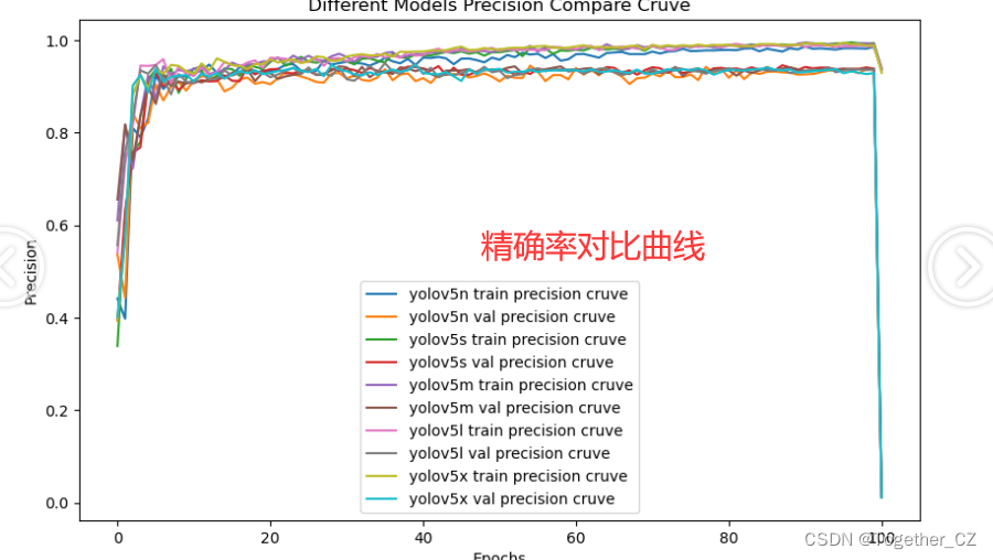
def plot_mc_curve(px, py, save_dir=Path('mc_curve.png'), names=(), xlabel='Confidence', ylabel='Metric'):"""Metric-confidence curve"""fig, ax = plt.subplots(1, 1, figsize=(9, 6), tight_layout=True)if 0 < len(names) < 21:  # display per-class legend if < 21 classesfor i, y in enumerate(py):ax.plot(px, y, linewidth=1, label=f'{names[i]}')  # plot(confidence, metric)else:ax.plot(px, py.T, linewidth=1, color='grey')  # plot(confidence, metric)y = smooth(py.mean(0), 0.05)ax.plot(px, y, linewidth=3, color='blue', label=f'all classes {y.max():.2f} at {px[y.argmax()]:.3f}')ax.set_xlabel(xlabel)ax.set_ylabel(ylabel)ax.set_xlim(0, 1)ax.set_ylim(0, 1)ax.legend(bbox_to_anchor=(1.04, 1), loc="upper left")ax.set_title(f'{ylabel}-Confidence Curve')fig.savefig(save_dir, dpi=250)plt.close(fig)def plot_pr_curve(px, py, ap, save_dir=Path('pr_curve.png'), names=()):"""Precision-recall curve"""fig, ax = plt.subplots(1, 1, figsize=(9, 6), tight_layout=True)py = np.stack(py, axis=1)if 0 < len(names) < 21:  # display per-class legend if < 21 classesfor i, y in enumerate(py.T):ax.plot(px, y, linewidth=1, label=f'{names[i]} {ap[i, 0]:.3f}')  # plot(recall, precision)else:ax.plot(px, py, linewidth=1, color='grey')  # plot(recall, precision)ax.plot(px, py.mean(1), linewidth=3, color='blue', label='all classes %.3f mAP@0.5' % ap[:, 0].mean())ax.set_xlabel('Recall')ax.set_ylabel('Precision')ax.set_xlim(0, 1)ax.set_ylim(0, 1)ax.legend(bbox_to_anchor=(1.04, 1), loc="upper left")ax.set_title('Precision-Recall Curve')fig.savefig(save_dir, dpi=250)plt.close(fig)def ap_per_class(tp, conf, pred_cls, target_cls, plot=False, save_dir='.', names=(), eps=1e-16, prefix=""):""" Compute the average precision, given the recall and precision curves.Source: https://github.com/rafaelpadilla/Object-Detection-Metrics.# Argumentstp:  True positives (nparray, nx1 or nx10).conf:  Objectness value from 0-1 (nparray).pred_cls:  Predicted object classes (nparray).target_cls:  True object classes (nparray).plot:  Plot precision-recall curve at mAP@0.5save_dir:  Plot save directory# ReturnsThe average precision as computed in py-faster-rcnn."""# Sort by objectnessi = np.argsort(-conf)tp, conf, pred_cls = tp[i], conf[i], pred_cls[i]# Find unique classesunique_classes, nt = np.unique(target_cls, return_counts=True)nc = unique_classes.shape[0]  # number of classes, number of detections# Create Precision-Recall curve and compute AP for each classpx, py = np.linspace(0, 1, 1000), []  # for plottingap, p, r = np.zeros((nc, tp.shape[1])), np.zeros((nc, 1000)), np.zeros((nc, 1000))for ci, c in enumerate(unique_classes):i = pred_cls == cn_l = nt[ci]  # number of labelsn_p = i.sum()  # number of predictionsif n_p == 0 or n_l == 0:continue# Accumulate FPs and TPsfpc = (1 - tp[i]).cumsum(0)tpc = tp[i].cumsum(0)# Recallrecall = tpc / (n_l + eps)  # recall curver[ci] = np.interp(-px, -conf[i], recall[:, 0], left=0)  # negative x, xp because xp decreases# Precisionprecision = tpc / (tpc + fpc)  # precision curvep[ci] = np.interp(-px, -conf[i], precision[:, 0], left=1)  # p at pr_score# AP from recall-precision curvefor j in range(tp.shape[1]):ap[ci, j], mpre, mrec = compute_ap(recall[:, j], precision[:, j])if plot and j == 0:py.append(np.interp(px, mrec, mpre))  # precision at mAP@0.5# Compute F1 (harmonic mean of precision and recall)f1 = 2 * p * r / (p + r + eps)names = [v for k, v in names.items() if k in unique_classes]  # list: only classes that have datanames = dict(enumerate(names))  # to dictif plot:plot_pr_curve(px, py, ap, Path(save_dir) / f'{prefix}PR_curve.png', names)plot_mc_curve(px, f1, Path(save_dir) / f'{prefix}F1_curve.png', names, ylabel='F1')plot_mc_curve(px, p, Path(save_dir) / f'{prefix}P_curve.png', names, ylabel='Precision')plot_mc_curve(px, r, Path(save_dir) / f'{prefix}R_curve.png', names, ylabel='Recall')i = smooth(f1.mean(0), 0.1).argmax()  # max F1 indexp, r, f1 = p[:, i], r[:, i], f1[:, i]tp = (r * nt).round()  # true positivesfp = (tp / (p + eps) - tp).round()  # false positivesreturn tp, fp, p, r, f1, ap, unique_classes.astype(int)class Annotator:# YOLOv5 Annotator for train/val mosaics and jpgs and detect/hub inference annotationsdef __init__(self, im, line_width=None, font_size=None, font='Arial.ttf', pil=False, example='abc'):assert im.data.contiguous, 'Image not contiguous. Apply np.ascontiguousarray(im) to Annotator() input images.'non_ascii = not is_ascii(example)  # non-latin labels, i.e. asian, arabic, cyrillicself.pil = pil or non_asciiif self.pil:  # use PILself.im = im if isinstance(im, Image.Image) else Image.fromarray(im)self.draw = ImageDraw.Draw(self.im)self.font = check_pil_font(font='Arial.Unicode.ttf' if non_ascii else font,size=font_size or max(round(sum(self.im.size) / 2 * 0.035), 12))else:  # use cv2self.im = imself.lw = line_width or max(round(sum(im.shape) / 2 * 0.003), 2)  # line widthdef box_label(self, box, label='', color=(128, 128, 128), txt_color=(255, 255, 255)):# Add one xyxy box to image with labelif self.pil or not is_ascii(label):self.draw.rectangle(box, width=self.lw, outline=color)  # boxif label:w, h = self.font.getsize(label)  # text width, heightoutside = box[1] - h >= 0  # label fits outside boxself.draw.rectangle((box[0], box[1] - h if outside else box[1], box[0] + w + 1,box[1] + 1 if outside else box[1] + h + 1),fill=color,)# self.draw.text((box[0], box[1]), label, fill=txt_color, font=self.font, anchor='ls')  # for PIL>8.0self.draw.text((box[0], box[1] - h if outside else box[1]), label, fill=txt_color, font=self.font)else:  # cv2p1, p2 = (int(box[0]), int(box[1])), (int(box[2]), int(box[3]))cv2.rectangle(self.im, p1, p2, color, thickness=self.lw, lineType=cv2.LINE_AA)if label:tf = max(self.lw - 1, 1)  # font thicknessw, h = cv2.getTextSize(label, 0, fontScale=self.lw / 3, thickness=tf)[0]  # text width, heightoutside = p1[1] - h >= 3p2 = p1[0] + w, p1[1] - h - 3 if outside else p1[1] + h + 3cv2.rectangle(self.im, p1, p2, color, -1, cv2.LINE_AA)  # filledcv2.putText(self.im,label, (p1[0], p1[1] - 2 if outside else p1[1] + h + 2),0,self.lw / 3,txt_color,thickness=tf,lineType=cv2.LINE_AA)def masks(self, masks, colors, im_gpu, alpha=0.5, retina_masks=False):"""Plot masks at once.Args:masks (tensor): predicted masks on cuda, shape: [n, h, w]colors (List[List[Int]]): colors for predicted masks, [[r, g, b] * n]im_gpu (tensor): img is in cuda, shape: [3, h, w], range: [0, 1]alpha (float): mask transparency: 0.0 fully transparent, 1.0 opaque"""if self.pil:# convert to numpy firstself.im = np.asarray(self.im).copy()if len(masks) == 0:self.im[:] = im_gpu.permute(1, 2, 0).contiguous().cpu().numpy() * 255colors = torch.tensor(colors, device=im_gpu.device, dtype=torch.float32) / 255.0colors = colors[:, None, None]  # shape(n,1,1,3)masks = masks.unsqueeze(3)  # shape(n,h,w,1)masks_color = masks * (colors * alpha)  # shape(n,h,w,3)inv_alph_masks = (1 - masks * alpha).cumprod(0)  # shape(n,h,w,1)mcs = (masks_color * inv_alph_masks).sum(0) * 2  # mask color summand shape(n,h,w,3)im_gpu = im_gpu.flip(dims=[0])  # flip channelim_gpu = im_gpu.permute(1, 2, 0).contiguous()  # shape(h,w,3)im_gpu = im_gpu * inv_alph_masks[-1] + mcsim_mask = (im_gpu * 255).byte().cpu().numpy()self.im[:] = im_mask if retina_masks else scale_image(im_gpu.shape, im_mask, self.im.shape)if self.pil:# convert im back to PIL and update drawself.fromarray(self.im)def rectangle(self, xy, fill=None, outline=None, width=1):# Add rectangle to image (PIL-only)self.draw.rectangle(xy, fill, outline, width)def text(self, xy, text, txt_color=(255, 255, 255), anchor='top'):# Add text to image (PIL-only)if anchor == 'bottom':  # start y from font bottomw, h = self.font.getsize(text)  # text width, heightxy[1] += 1 - hself.draw.text(xy, text, fill=txt_color, font=self.font)def fromarray(self, im):# Update self.im from a numpy arrayself.im = im if isinstance(im, Image.Image) else Image.fromarray(im)self.draw = ImageDraw.Draw(self.im)def result(self):# Return annotated image as arrayreturn np.asarray(self.im)def plot_lr_scheduler(optimizer, scheduler, epochs=300, save_dir=''):# Plot LR simulating training for full epochsoptimizer, scheduler = copy(optimizer), copy(scheduler)  # do not modify originalsy = []for _ in range(epochs):scheduler.step()y.append(optimizer.param_groups[0]['lr'])plt.plot(y, '.-', label='LR')plt.xlabel('epoch')plt.ylabel('LR')plt.grid()plt.xlim(0, epochs)plt.ylim(0)plt.savefig(Path(save_dir) / 'LR.png', dpi=200)plt.close()def plot_labels(labels, names=(), save_dir=Path('')):# plot dataset labelsLOGGER.info(f"Plotting labels to {save_dir / 'labels.jpg'}... ")c, b = labels[:, 0], labels[:, 1:].transpose()  # classes, boxesnc = int(c.max() + 1)  # number of classesx = pd.DataFrame(b.transpose(), columns=['x', 'y', 'width', 'height'])# seaborn correlogramsn.pairplot(x, corner=True, diag_kind='auto', kind='hist', diag_kws=dict(bins=50), plot_kws=dict(pmax=0.9))plt.savefig(save_dir / 'labels_correlogram.jpg', dpi=200)plt.close()# matplotlib labelsmatplotlib.use('svg')  # fasterax = plt.subplots(2, 2, figsize=(8, 8), tight_layout=True)[1].ravel()y = ax[0].hist(c, bins=np.linspace(0, nc, nc + 1) - 0.5, rwidth=0.8)with contextlib.suppress(Exception):  # color histogram bars by class[y[2].patches[i].set_color([x / 255 for x in colors(i)]) for i in range(nc)]  # known issue #3195ax[0].set_ylabel('instances')if 0 < len(names) < 30:ax[0].set_xticks(range(len(names)))ax[0].set_xticklabels(list(names.values()), rotation=90, fontsize=10)else:ax[0].set_xlabel('classes')sn.histplot(x, x='x', y='y', ax=ax[2], bins=50, pmax=0.9)sn.histplot(x, x='width', y='height', ax=ax[3], bins=50, pmax=0.9)# rectangleslabels[:, 1:3] = 0.5  # centerlabels[:, 1:] = xywh2xyxy(labels[:, 1:]) * 2000img = Image.fromarray(np.ones((2000, 2000, 3), dtype=np.uint8) * 255)for cls, *box in labels[:1000]:ImageDraw.Draw(img).rectangle(box, width=1, outline=colors(cls))  # plotax[1].imshow(img)ax[1].axis('off')for a in [0, 1, 2, 3]:for s in ['top', 'right', 'left', 'bottom']:ax[a].spines[s].set_visible(False)plt.savefig(save_dir / 'labels.jpg', dpi=200)matplotlib.use('Agg')plt.close()def plot_results(file='path/to/results.csv', dir=''):# Plot training results.csv. Usage: from utils.plots import *; plot_results('path/to/results.csv')save_dir = Path(file).parent if file else Path(dir)fig, ax = plt.subplots(2, 5, figsize=(12, 6), tight_layout=True)ax = ax.ravel()files = list(save_dir.glob('results*.csv'))assert len(files), f'No results.csv files found in {save_dir.resolve()}, nothing to plot.'for f in files:try:data = pd.read_csv(f)s = [x.strip() for x in data.columns]x = data.values[:, 0]for i, j in enumerate([1, 2, 3, 4, 5, 8, 9, 10, 6, 7]):y = data.values[:, j].astype('float')# y[y == 0] = np.nan  # don't show zero valuesax[i].plot(x, y, marker='.', label=f.stem, linewidth=2, markersize=8)ax[i].set_title(s[j], fontsize=12)# if j in [8, 9, 10]:  # share train and val loss y axes#     ax[i].get_shared_y_axes().join(ax[i], ax[i - 5])except Exception as e:LOGGER.info(f'Warning: Plotting error for {f}: {e}')ax[1].legend()fig.savefig(save_dir / 'results.png', dpi=200)plt.close()

【Precision曲线】
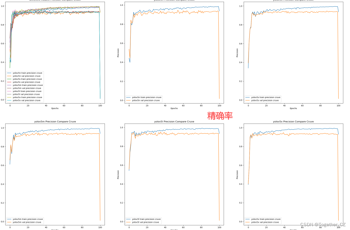
精确率曲线（Precision-Recall Curve）是一种用于评估二分类模型在不同阈值下的精确率性能的可视化工具。它通过绘制不同阈值下的精确率和召回率之间的关系图来帮助我们了解模型在不同阈值下的表现。
精确率（Precision）是指被正确预测为正例的样本数占所有预测为正例的样本数的比例。召回率（Recall）是指被正确预测为正例的样本数占所有实际为正例的样本数的比例。
绘制精确率曲线的步骤如下：
使用不同的阈值将预测概率转换为二进制类别标签。通常，当预测概率大于阈值时，样本被分类为正例，否则分类为负例。
对于每个阈值，计算相应的精确率和召回率。
将每个阈值下的精确率和召回率绘制在同一个图表上，形成精确率曲线。
根据精确率曲线的形状和变化趋势，可以选择适当的阈值以达到所需的性能要求。
通过观察精确率曲线，我们可以根据需求确定最佳的阈值，以平衡精确率和召回率。较高的精确率意味着较少的误报，而较高的召回率则表示较少的漏报。根据具体的业务需求和成本权衡，可以在曲线上选择合适的操作点或阈值。
精确率曲线通常与召回率曲线（Recall Curve）一起使用，以提供更全面的分类器性能分析，并帮助评估和比较不同模型的性能。

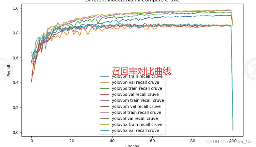
【Recall曲线】
召回率曲线（Recall Curve）是一种用于评估二分类模型在不同阈值下的召回率性能的可视化工具。它通过绘制不同阈值下的召回率和对应的精确率之间的关系图来帮助我们了解模型在不同阈值下的表现。
召回率（Recall）是指被正确预测为正例的样本数占所有实际为正例的样本数的比例。召回率也被称为灵敏度（Sensitivity）或真正例率（True Positive Rate）。
绘制召回率曲线的步骤如下：
使用不同的阈值将预测概率转换为二进制类别标签。通常，当预测概率大于阈值时，样本被分类为正例，否则分类为负例。
对于每个阈值，计算相应的召回率和对应的精确率。
将每个阈值下的召回率和精确率绘制在同一个图表上，形成召回率曲线。
根据召回率曲线的形状和变化趋势，可以选择适当的阈值以达到所需的性能要求。
通过观察召回率曲线，我们可以根据需求确定最佳的阈值，以平衡召回率和精确率。较高的召回率表示较少的漏报，而较高的精确率意味着较少的误报。根据具体的业务需求和成本权衡，可以在曲线上选择合适的操作点或阈值。
召回率曲线通常与精确率曲线（Precision Curve）一起使用，以提供更全面的分类器性能分析，并帮助评估和比较不同模型的性能。

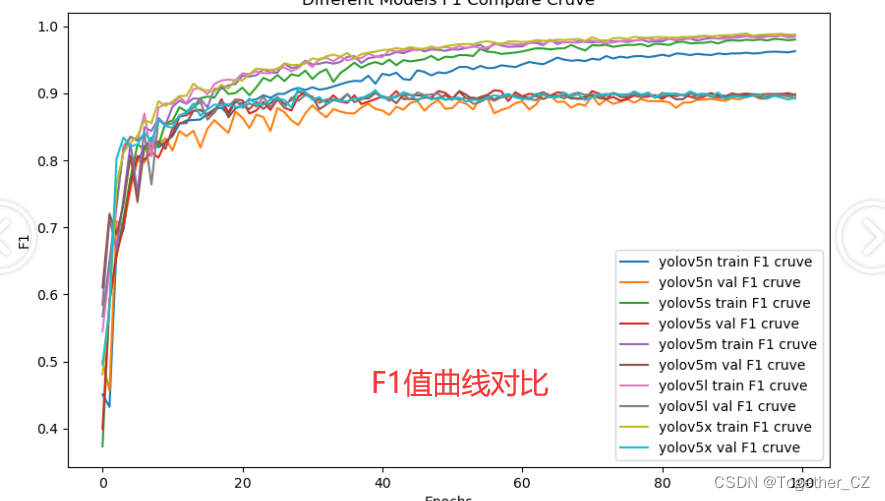
【F1值曲线】
F1值曲线是一种用于评估二分类模型在不同阈值下的性能的可视化工具。它通过绘制不同阈值下的精确率（Precision）、召回率（Recall）和F1分数的关系图来帮助我们理解模型的整体性能。
F1分数是精确率和召回率的调和平均值，它综合考虑了两者的性能指标。F1值曲线可以帮助我们确定在不同精确率和召回率之间找到一个平衡点，以选择最佳的阈值。
绘制F1值曲线的步骤如下：
使用不同的阈值将预测概率转换为二进制类别标签。通常，当预测概率大于阈值时，样本被分类为正例，否则分类为负例。
对于每个阈值，计算相应的精确率、召回率和F1分数。
将每个阈值下的精确率、召回率和F1分数绘制在同一个图表上，形成F1值曲线。
根据F1值曲线的形状和变化趋势，可以选择适当的阈值以达到所需的性能要求。
F1值曲线通常与接收者操作特征曲线（ROC曲线）一起使用，以帮助评估和比较不同模型的性能。它们提供了更全面的分类器性能分析，可以根据具体应用场景来选择合适的模型和阈值设置。

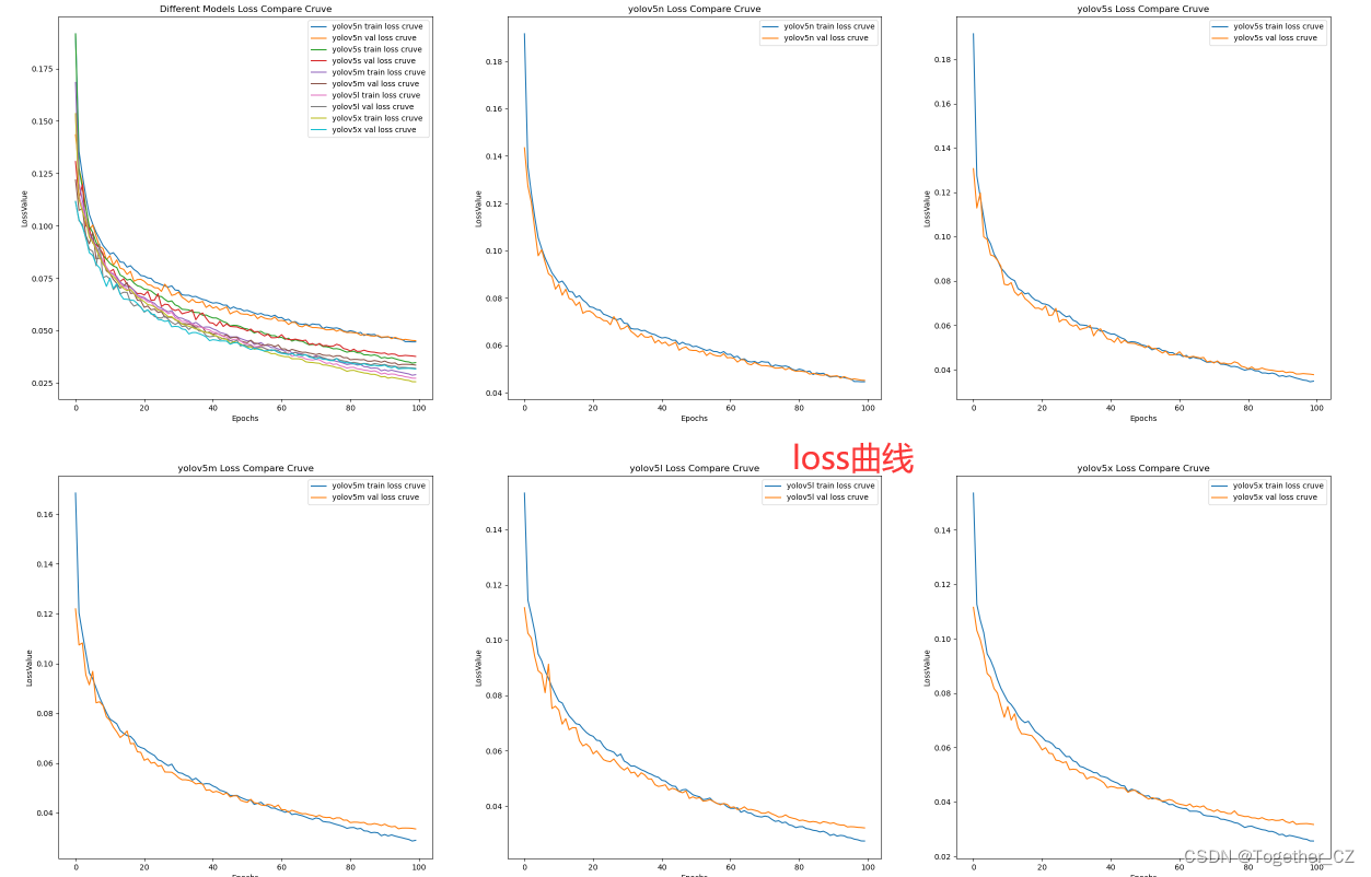
【loss对比曲线】

上面是从单个指标的维度来横向地对比不同模型的表现能力，通过自由的组合上述的指标数据提取和可视化部分代码，可以得到更为全面的实现，如下所示：

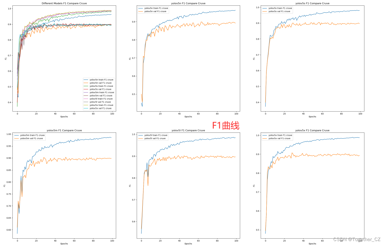
【F1值曲线】

【loss曲线】

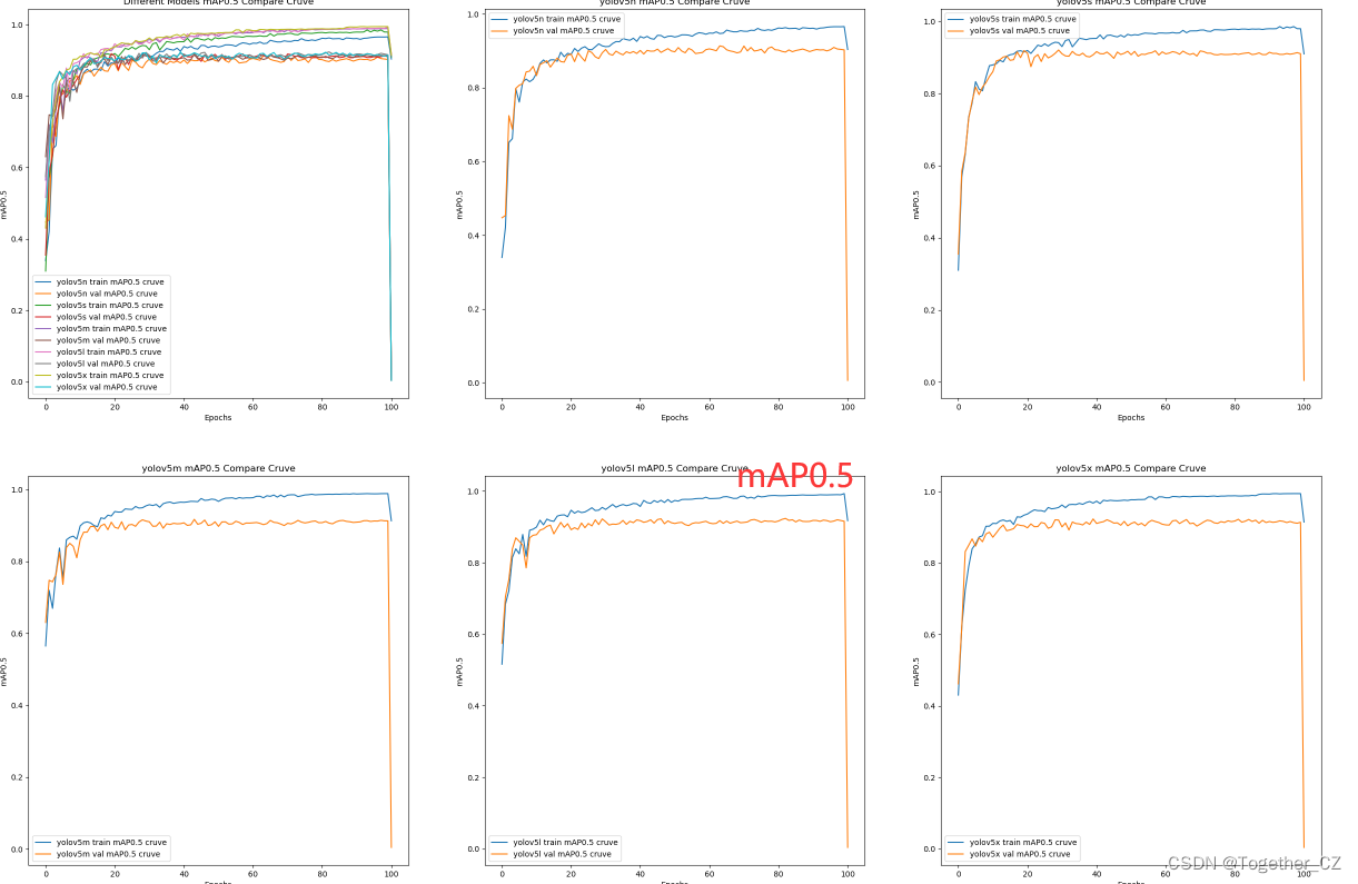
【mAP0.5曲线】

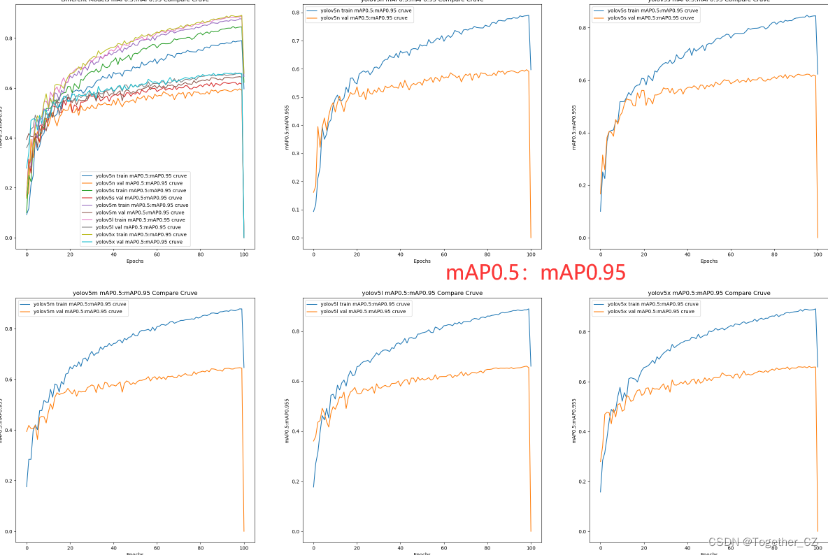
【mAP0.5：mAP0.95曲线】

【precision曲线】

【recall曲线】

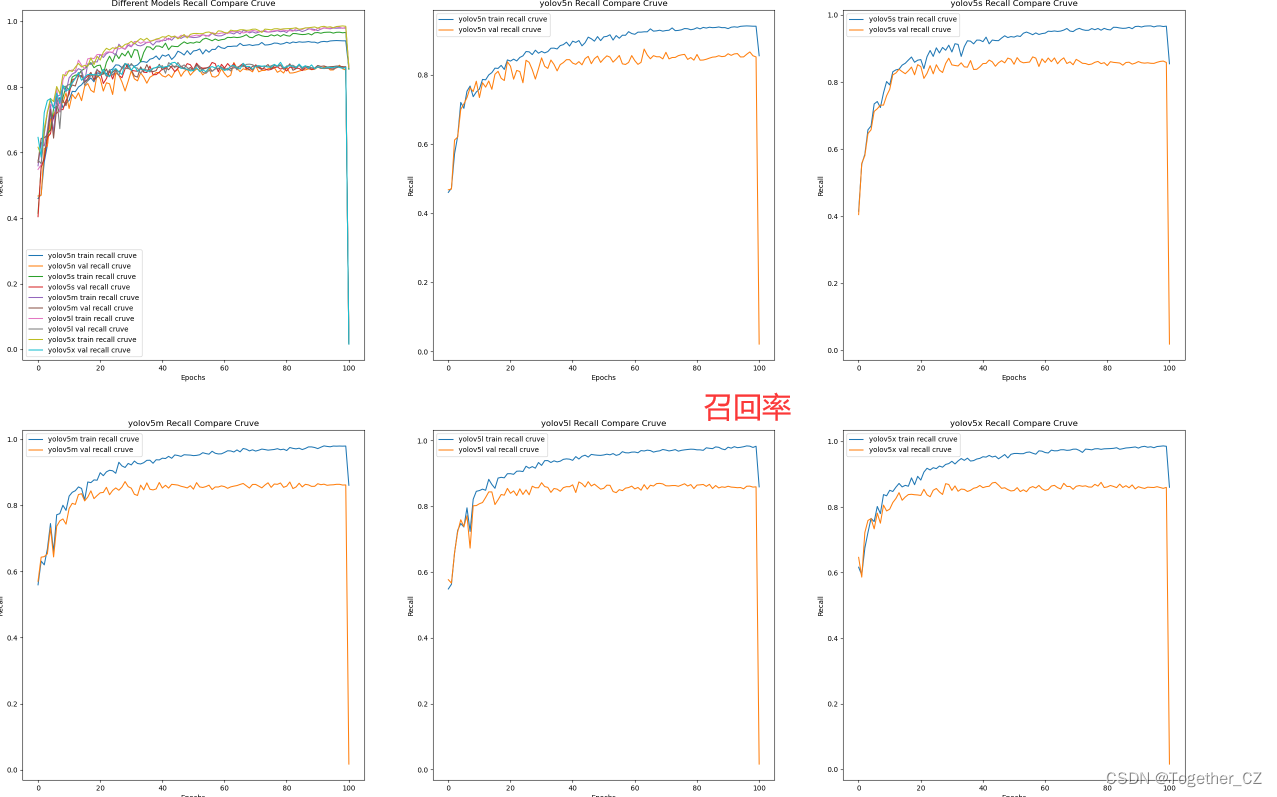
整体来看：n系列的结果最差，s系列次之，m系列和l、x系列没有很明显的差距，但m系列的模型在边缘端设备部署的时候有性能和推理速度的优势，最终落地选择的是m系列的模型，我们还尝试了以m系列为基准集成了一些tricks进行性能的提升优化处理，另外还做了一些相应的轻量化处理工作，后面有时间的话再通过博文记录吧。