1. 引言 📌

在这里插入图片描述

参加这场比赛的时间，应该是还剩一个月不到了，本来没啥想法，因为在忙一些其它的比赛或者是工作和个人上的烦心事，不过在看过了赛题分析后，整体给我感观是一道挺有意思的学习赛，不仅仅是它的限时2小时，不允许用GPU进行推理，在这之前，前面几年都有对鸟类叫声开展了一系列的research，是的，这是研究类性质的比赛，因此在前面几年积累下了很多的资料文献，而在今年，玩法和数据多样性上进行了更新，我也看到其中一个competition HOST在discussion说去年一年他又收集到多少珍稀鸟类物种的叫声，最近在研究怎么将GPT4带入这项研究中，以及整个HOST团队的自我介绍，这让我感觉很cool，可以一试，虽然最终只拿到了铜牌，最后的private还掉了波分，原因是我没搞清楚切榜后我标的次best score咋没生效，少了4个千分位，但最终还是受益匪浅，以下是我的一个总结。

2. 📊EDA 📊

2.1 声音频率指标介绍 🔉🔉

因为声音就是鸟的叫声，格式为ogg音频，评测指标为mAP，加上一些额外要求，整个都很明确直观，所以直接进行eda，首先针对一个文件去可视化它的声音与波段，比如：

def load_audio(filepath, sr=32000, normalize=True):audio, orig_sr = librosa.load(filepath, sr=None)if sr!=orig_sr:audio = librosa.resample(y, orig_sr, sr)audio = audio.astype('float32').ravel()audio = tf.convert_to_tensor(audio)return audiodef display_audio(row):# Caption for vizcaption = f'Id: {row.filename}'# Read audio fileaudio = load_audio(row.filepath)# Keep fixed length audioaudio = audio[:CFG.audio_len]# Display audioprint("# Audio:")display(ipd.Audio(audio.numpy(), rate=CFG.sample_rate))print('# Visualization:')plt.figure(figsize=(12, 3))plt.title(caption)# Waveplotlid.waveshow(audio.numpy(),sr=CFG.sample_rate,)plt.xlabel('');plt.show()display_audio(test_df.iloc[0])

在这里插入图片描述

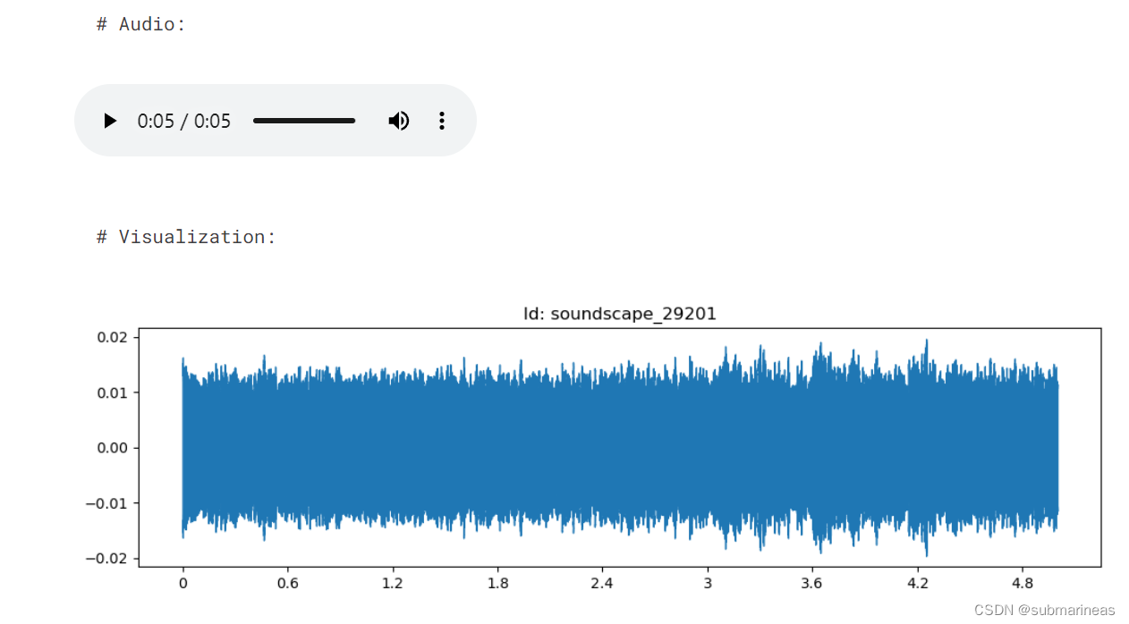
在jupyter notebook中一般能直接播放该音频，算是librosa做了相应的兼容，然后将声音波段不加任何处理直接画出，可以看出来很嘈杂，主要没有调节频率，也没有提取出特征，所以更进一步的还有Spectograms（光谱图）、Mel Spectograms（梅尔光/频谱）、Chromagram（色谱图）、MFCC（Mel Frequency Cepstral Coefficients）等等，这里做一个大致解释为：

Waveforms：在音频处理中，波形是声音信号的图形表示，显示了信号随时间的变化。它是 y 轴上声波振幅与 x 轴上时间的关系图。波形可以用来显示和分析音频信号的特性，如频率、幅度、相位和持续时间。
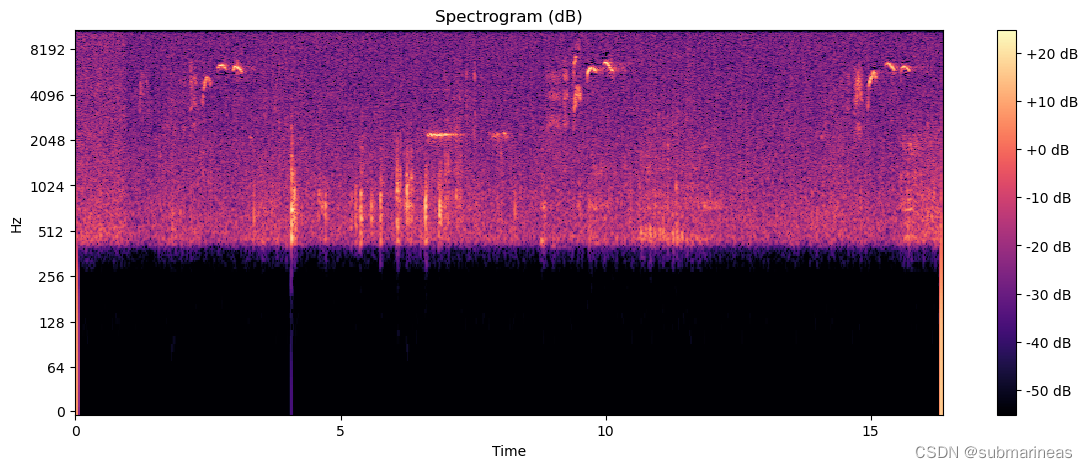
Spectograms：光谱图是声音或其他信号的频谱随时间变化的可视化表示。这是一种分析声音信号的方法，以了解信号如何随着时间的推移而变化，以及在任何给定的时间点，信号中存在哪些频率。光谱图的 x 轴代表时间，而 y 轴代表频率。光谱图中每个点的颜色或亮度的强度代表该时间点频率的振幅或能量。
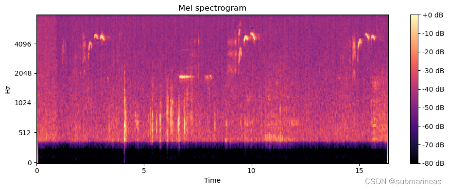
Mel Spectograms：梅尔谱图是一种使用梅尔标度来确定频率箱间距的谱图。梅尔音阶是一种感知音高的音阶，被听众判断为彼此之间的距离相等。通过使用梅尔音阶，频率箱在较低频率时间隔得更近，在较高频率时间隔得更远，这更符合人类感知声音的方式。
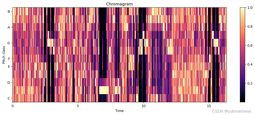
Chromagram：色谱图是音频信号的音高内容的可视化表示，其中每一列对应于一个特定的频带或音高类别。它是声音中能量分布的二维表示，绘制成时间和音高等级的函数。色谱图的计算方法是将音频信号的短时距傅里叶变换(STFT)投射到音高分类基础上，通常使用一组12个对数间隔的滤波器来表示西方音阶的12个音高分类。
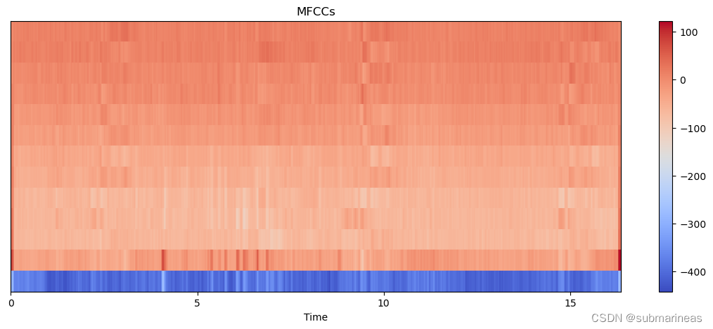
MFCC： MFCC 代表梅尔频率倒谱系数，这是一种常用于语音处理、音乐信息检索和其他相关领域的特征提取技术。 MFCC 来源于音频信号的短时距傅里叶变换(STFT) ，包括将信号分解成小的、重叠的片段，并在每个片段上执行一个傅里叶变换以获得其频谱。然后将梅尔音阶应用到频谱上，将其转换成接近人类听觉系统感知声音的对数尺度。

上面是根据wiki与高star的eda翻译而成，看起来文字有点多。就此写出完整代码为：

def audio_eda(audio_path):# Load an audio filesamples, sample_rate = librosa.load(audio_path)# Visualize the waveformplt.figure(figsize=(14, 5))librosa.display.waveshow(samples, sr=sample_rate)plt.title('Waveform')# Compute the spectrogramspectrogram = librosa.stft(samples)spectrogram_db = librosa.amplitude_to_db(abs(spectrogram))# Visualize the spectrogramplt.figure(figsize=(14, 5))librosa.display.specshow(spectrogram_db, sr=sample_rate, x_axis='time', y_axis='log')plt.colorbar(format='%+2.0f dB')plt.title('Spectrogram (dB)')# Compute the mel spectrogram# Visualize the mel spectrogramS = librosa.feature.melspectrogram(y=samples, sr=sample_rate)# Visualize mel spectrogramplt.figure(figsize=(10, 4))librosa.display.specshow(librosa.power_to_db(S, ref=np.max), y_axis='mel', fmax=8000, x_axis='time')plt.colorbar(format='%+2.0f dB')plt.title('Mel spectrogram')plt.tight_layout()# Compute the chromagramchromagram = librosa.feature.chroma_stft( y = samples , sr = sample_rate)# Visualize the chromagramplt.figure(figsize=(14, 5))librosa.display.specshow(chromagram, sr=sample_rate, x_axis='time', y_axis='chroma')plt.colorbar()plt.title('Chromagram')# Compute the MFCCsmfccs = librosa.feature.mfcc(y=samples, sr=sample_rate, n_mfcc=13)# Visualize the MFCCsplt.figure(figsize=(14, 5))librosa.display.specshow(mfccs, sr=sample_rate, x_axis='time')plt.colorbar()plt.title('MFCCs')# Show the plotsdisplay(Audio(samples, rate=sample_rate))plt.show()

2.1.1 African Gray Flycatcher 🐤

根据网络上的截图与现有的2023 dataset，可以选取African Gray Flycatcher 这种鸟类进行可视化，该品种的样子为：

在这里插入图片描述

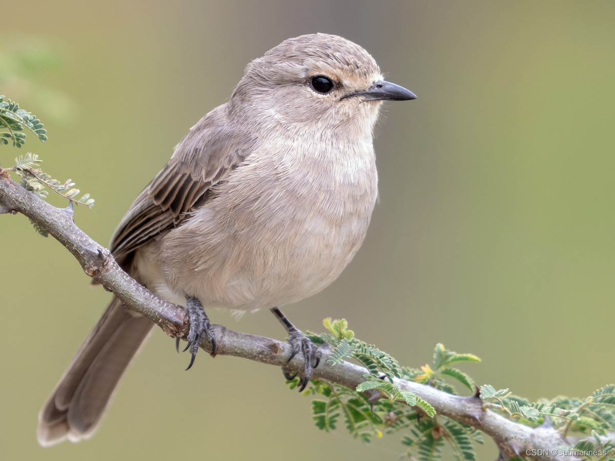
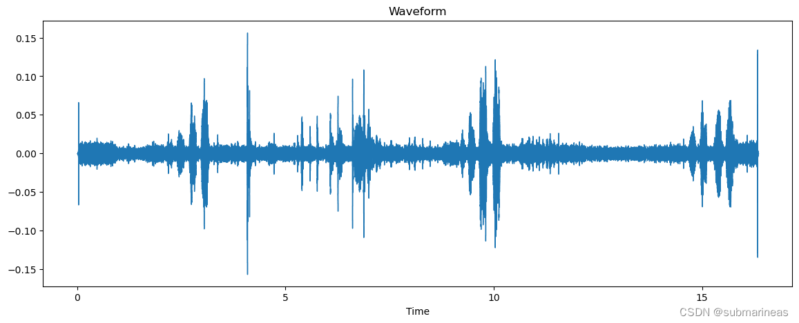
它是位于非洲的捕蝇鸟，标签为afgfly1，学名叫Bradornis microrhynchus，我们用它的标签位置，可直接进行分析：

audio_eda("/kaggle/input/birdclef-2023/train_audio/afgfly1/XC134487.ogg")

得到它的一个波段图：
在这里插入图片描述

针对原始音频进行librosa.stft（短时傅里叶变换），并可视化其以分贝为单位的光谱图：

在这里插入图片描述

通过librosa.feature.melspectrogram，计算音频信号的梅尔频谱，将计算结果可视化为：

在这里插入图片描述

通过librosa.feature.chroma_stft，计算音频信号的色度，将计算结果可视化为色谱图：

在这里插入图片描述

最后就是利用librosa.feature.mfcc计算音频信号的梅尔频率倒谱系数，这可以是后续扩增特征的强特，更常用于说话人识别、情感识别、音乐检索等任务，可视化为：
在这里插入图片描述

2.1.2 African Goshawk 🕊️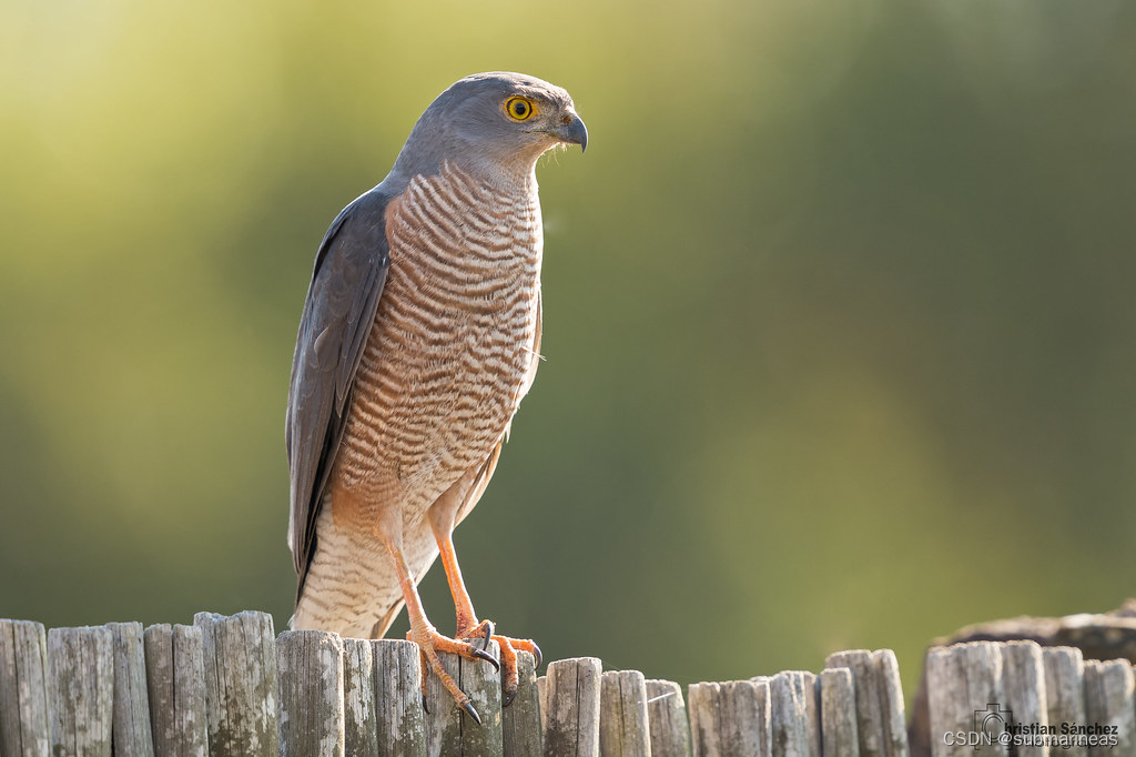

它的英文直译是非洲鹰，主要标签位于afrgos1，学名为Accipiter tachiro，我们同样可以用上面的方式进行可视化：

audio_eda("/kaggle/input/birdclef-2023/train_audio/afrgos1/XC115984.ogg")

当然，碍于篇幅就不再展示。减去这两种，还剩262种，里面有猛禽，比如说常见的秃鹰等，但大多还是小型的，比如非洲裸眼画眉、东非黑头黄鹂、金腰燕、柳莺等等。

2.2 birdclef train_metadata 分析 🎨

train_metadata.csv 为总的feature introduction，这里我发现了两种比较有意思的visual方式，第一种当然还是以pandas读入并做info：

trainmeta_df = pd.read_csv("/kaggle/input/birdclef-2023/train_metadata.csv")
trainmeta_df.info()

可得到每一feature的统计结果：

<class 'pandas.core.frame.DataFrame'>
RangeIndex: 16941 entries, 0 to 16940
Data columns (total 12 columns):#   Column            Non-Null Count  Dtype  
---  ------            --------------  -----  0   primary_label     16941 non-null  object 1   secondary_labels  16941 non-null  object 2   type              16941 non-null  object 3   latitude          16714 non-null  float644   longitude         16714 non-null  float645   scientific_name   16941 non-null  object 6   common_name       16941 non-null  object 7   author            16941 non-null  object 8   license           16941 non-null  object 9   rating            16941 non-null  float6410  url               16941 non-null  object 11  filename          16941 non-null  object 
dtypes: float64(3), object(9)
memory usage: 1.6+ MB
None

第二种方式就是利用skimpy.skim：

在这里插入图片描述

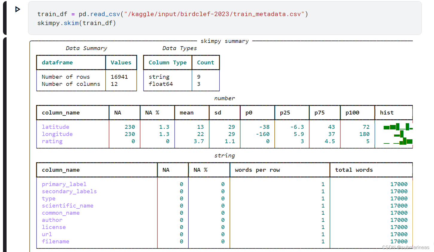
这种虽然与pandas的discribe差不多，但好处在于比较赏心悦目，表格皆可以复制出来，虽然对后续助力不大，因为它不是一个完整eda的包。

那根据上述统计，可以比较简单的得到三点信息：

经纬度有227个(1.34%)缺失值
经度和rating是倾斜的，即存在偏态或长尾分布
Primary labels , Secondary Labels , Type , Scientific Name , Common Name , Author ,Filename 暂时没发现什么问题，基数较大

针对Primary labels 指标再分析，可以看到它的一个分布情况：

fig = px.histogram(trainmeta_df, x="primary_label", nbins=len(trainmeta_df["primary_label"].unique()))
fig.update_layout(title_text="Distribution of Primary Labels")
fig.show()

在这里插入图片描述
虽然有二级标签，可主标签某种程度上，就对应了这264种鸟类的一个数据量的情况，能发现其极度的不平衡，不过作为多分类，整体分布还好，所以后续会对此进行采样以追求balance。

2.2.1 Map 🌍

上述的metatrain分析后，发现还提供了经纬度，那可以更进一步观察264种鸟类的栖息情况：

fig = px.scatter(trainmeta_df, x="longitude", y="latitude", color="common_name")
fig.update_layout(title="Distribution of Recordings by Location")
fig.show()

在这里插入图片描述

那再将它带入公开街道地图后，为：

fig = px.scatter_mapbox(trainmeta_df, lat="latitude", lon="longitude", color="common_name",hover_name="filename", hover_data=["common_name", "author", "rating"],zoom=3, height=500)
fig.update_layout(mapbox_style="open-street-map")
fig.update_layout(margin={"r":0,"t":0,"l":0,"b":0})
fig.show()

在这里插入图片描述
当然，还可以这些经纬度继续画其它的如地形图，直接反应于地势，或者改为3d图像，这里不再演示

3. baseline 🐦🎧📊

3.1 理论说明 📖

音频分类，其实简单来讲，可以说是根据梅尔频谱或者梅尔倒谱等方式将频率转化为图像，然后用卷积等方式加FC得到概率，大致的流程图为：

在这里插入图片描述

因为这部分代码较多，而且我所使用的Architecture是基于public中tensorflow的一个方案，中途把很少用的tensorflow 2.0语法回头看了下，自己尝试着修改，结果一堆bug，搞得我心态炸裂，就简单概括下。

我所使用的baseline，在我查阅了之前比赛经验事后了解到，应该是参照的这篇论文：PANNs: Large-Scale Pretrained Audio Neural Networks for
Audio Pattern Recognition

PANNs 是一种基于深度学习的音频识别框架，论文中它所写得一个步骤为：

预处理：将音频信号转换为时频图像，例如使用短时傅里叶变换（STFT）。
特征提取：使用卷积神经网络（CNN）和循环神经网络（RNN）等技术来提取音频特征。
预训练：在大规模数据集上训练模型，例如使用Google的AudioSet数据集。
微调：将预训练模型迁移到新的任务中进行微调，例如在ESC-50、MSOS、RAVDESS、DCASE 2018 Task 2和GTZAN等任务中进行微调。
测试和评估：对微调后的模型进行测试和评估，例如计算准确率、召回率等指标。

总体来说，PANNs的流程是先在大规模数据集上预训练模型，然后将其迁移到新的任务中进行微调。这种方法可以显著提高音频识别任务的性能，事实上确实如此，这当然不仅仅是音频领域，其它也适用。而正是基于它的这种架构，也被之后称为了SED（Sound Event Detection）model ，即：

在这里插入图片描述

但我并没有使用该架构，第一是时间问题，第二是源码基于pytorch的，而我后期用tensorflow复现后与本身的baseline有冲突，很奇怪，就没用了。

3.2 数据切分 🔪

# Import required packages
from sklearn.model_selection import StratifiedKFold# Initialize the StratifiedKFold object with 5 splits and shuffle the data
skf1 = StratifiedKFold(n_splits=25, shuffle=True, random_state=CFG.seed)
skf2 = StratifiedKFold(n_splits=CFG.num_fold, shuffle=True, random_state=CFG.seed)# Reset the index of the dataframe
df_pre = df_pre.reset_index(drop=True)
df_23 = df_23.reset_index(drop=True)# Create a new column in the dataframe to store the fold number for each row
df_pre["fold"] = -1
df_23["fold"] = -1# BirdCLEF - 21 & 22
for fold, (train_idx, val_idx) in enumerate(skf1.split(df_pre, df_pre['primary_label'])):df_pre.loc[val_idx, 'fold'] = fold# IBirdCLEF - 23
for fold, (train_idx, val_idx) in enumerate(skf2.split(df_23, df_23['primary_label'])):df_23.loc[val_idx, 'fold'] = fold

优选5折 or 10折，按字段来进行分割，这不用多说。而因为我们还需要做pretrain，所以选用了birdclef 2020到2022年的数据，以及额外的官方数据集，与birdclef 2023区分开。

3.3 Filter & Upsample Data ⬆️

Filter：由于有些类甚至只有一个示例，我们需要使用过滤来确保它们在train data中。即通过始终将它们保存在train data中，并对其余数据进行交叉验证来实现这一点。
Upsample：上采样，针对很少类别的数据量提高其抽样率，来达到缓解“长尾”问题。
Downsample ：确保类的最大样本数。

def filter_data(df, thr=5):# Count the number of samples for each classcounts = df.primary_label.value_counts()# Condition that selects classes with less than `thr` samplescond = df.primary_label.isin(counts[counts<thr].index.tolist())# Add a new column to select samples for cross validationdf['cv'] = True# Set cv = False for those class where there is samples less than thrdf.loc[cond, 'cv'] = False# Return the filtered dataframereturn dfdef upsample_data(df, thr=20):# get the class distributionclass_dist = df['primary_label'].value_counts()# identify the classes that have less than the threshold number of samplesdown_classes = class_dist[class_dist < thr].index.tolist()# create an empty list to store the upsampled dataframesup_dfs = []# loop through the undersampled classes and upsample themfor c in down_classes:# get the dataframe for the current classclass_df = df.query("primary_label==@c")# find number of samples to addnum_up = thr - class_df.shape[0]# upsample the dataframeclass_df = class_df.sample(n=num_up, replace=True, random_state=CFG.seed)# append the upsampled dataframe to the listup_dfs.append(class_df)# concatenate the upsampled dataframes and the original dataframeup_df = pd.concat([df] + up_dfs, axis=0, ignore_index=True)return up_df

利用filter data可以得到相对完整的split data：

在这里插入图片描述

同样，得到上下采样后的数据集一个分布情况：

在这里插入图片描述

3.4 Data Augmentation 🌈

关于Data Augmentation（数据增强），有一些需要注意的点，即使可以将音频作为图像(光谱图)进行训练，但不能使用如水平翻转、旋转、剪切等计算机视觉的手段，因为它可能会污染图像(光谱图)中包含的信息，那这里比较推荐的两种方式为：

AudioAug：将音频直接应用于音频数据的增强。例如: 高斯噪声，Random CropPad，CutMix 和 MixUp
SpecAug：应用于光谱图数据的增强。

# Import required packages
import tensorflow_extra as tfe# Randomly shift audio -> any sound at <t> time may get shifted to <t+shift> time
@tf.function
def TimeShift(audio, prob=0.5):# Randomly apply time shift with probability `prob`if random_float() < prob:# Calculate random shift valueshift = random_int(shape=[], minval=0, maxval=tf.shape(audio)[0])# Randomly set the shift to be negative with 50% probabilityif random_float() < 0.5:shift = -shift# Roll the audio signal by the shift valueaudio = tf.roll(audio, shift, axis=0)return audio# Apply random noise to audio data
@tf.function
def GaussianNoise(audio, std=[0.0025, 0.025], prob=0.5):# Select a random value of standard deviation for Gaussian noise within the given rangestd = random_float([], std[0], std[1])# Randomly apply Gaussian noise with probability `prob`if random_float() < prob:# Add random Gaussian noise to the audio signalGN = tf.keras.layers.GaussianNoise(stddev=std)audio = GN(audio, training=True) # training=False don't apply noise to datareturn audio# Applies augmentation to Audio Signal
def AudioAug(audio):# Apply time shift and Gaussian noise to the audio signalaudio = TimeShift(audio, prob=CFG.timeshift_prob)audio = GaussianNoise(audio, prob=CFG.gn_prob)return audio# CutMix & MixUp
mixup_layer = tfe.layers.MixUp(alpha=CFG.mixup_alpha, prob=CFG.mixup_prob)
cutmix_layer = tfe.layers.CutMix(alpha=CFG.cutmix_alpha, prob=CFG.cutmix_prob)def CutMixUp(audios, labels):audios, labels = mixup_layer(audios, labels, training=True)audios, labels = cutmix_layer(audios, labels, training=True)return audios, labels

3.5 Loss, Metric & Optmizer 📉

关于dataloader的构建这里略过，我看中间主要利用了tensorflow的tf.data，这种pipeline的构建方式有点复杂，用了很多tensorflow新版本中的语法，我没完全看懂，但大受震撼，整体来讲，就是加了很多设置项，组成batch_size的形式批量推理，并能优化下一批推理的过程。但就我整体体验下来，还是很慢，emmm。。。

对于loss来讲，baseline使用了一个不同寻常的指标，即分类交叉熵(CCE)损失优化。该损失函数为：
$-\frac{1}{N} \sum_{i=1}^{N} \sum_{j=1}^{C} y_{i,j} \log(p_{i,j})$

该指标根据框架中作者的表述，是考虑到有些样本没有正样本，而增加真实阳性类别的概率，并减轻阳性类别非常少的物种的影响。在我之后的实验中，该指标确实有用，但作用也没有说的那么大，主要是tensorflow中可以直接引入：

def get_metrics():
#     acc = tf.keras.metrics.BinaryAccuracy(name='acc')auc = tf.keras.metrics.AUC(curve='PR', name='auc', multi_label=False) # auc on prcision-recall curveacc = tf.keras.metrics.CategoricalAccuracy(name='acc')return [acc, auc]def padded_cmap(y_true, y_pred, padding_factor=5):num_classes = y_true.shape[1]pad_rows = np.array([[1]*num_classes]*padding_factor)y_true = np.concatenate([y_true, pad_rows])y_pred = np.concatenate([y_pred, pad_rows])score = sklearn.metrics.average_precision_score(y_true, y_pred, average='macro',)return scoredef get_loss():if CFG.loss=="CCE":loss = tf.keras.losses.CategoricalCrossentropy(label_smoothing=CFG.label_smoothing)elif CFG.loss=="BCE":loss = tf.keras.losses.BinaryCrossentropy(label_smoothing=CFG.label_smoothing)else:raise ValueError("Loss not found")return loss

3.6 Modeling 🤖

import efficientnet.tfkeras as efn
import tensorflow_extra as tfe# Will download and load pretrained imagenet weights.
def build_model(CFG, model_name=None, num_classes=264, compile_model=True):"""Builds and returns a model based on the specified configuration."""# Create an input layer for the modelinp = tf.keras.layers.Input(shape=(None,))# Spectrogramout = tfe.layers.MelSpectrogram(n_mels=CFG.img_size[0],n_fft=CFG.nfft,hop_length=CFG.hop_length, sr=CFG.sample_rate,ref=1.0,out_channels=3)(inp)# Normalizeout = tfe.layers.ZScoreMinMax()(out)# TimeFreqMaskout = tfe.layers.TimeFreqMask(freq_mask_prob=0.5,num_freq_masks=1,freq_mask_param=10,time_mask_prob=0.5,num_time_masks=2,time_mask_param=25,time_last=False,)(out)# Load backbone modelbase = getattr(efn, model_name)(input_shape=(None, None, 3),include_top=0,weights=CFG.pretrain,fsr=CFG.fsr)# Pass the input through the base modelout = base(out)out = tf.keras.layers.GlobalAveragePooling2D()(out)out = tf.keras.layers.Dense(num_classes, activation='softmax')(out)model = tf.keras.models.Model(inputs=inp, outputs=out)if compile_model:# Set the optimizeropt = get_optimizer()# Set the loss functionloss = get_loss()# Set the evaluation metricsmetrics = get_metrics()# Compile the model with the specified optimizer, loss function, and metricsmodel.compile(optimizer=opt, loss=loss, metrics=metrics)return model

该模型构建得很简单，主要是因为推理时间受限，但用的库又是些之前没听说过的，比如说tensorflow_extra，在我后续优化该模型时，这个库还是有挺多坑的。那这里可以summary输出模型结构为：

Model: "model"
_________________________________________________________________Layer (type)                Output Shape              Param #   
=================================================================input_1 (InputLayer)        [(None, None)]            0         mel_spectrogram (MelSpectro  (None, 128, None, 3)     0         gram)                                                           z_score_min_max (ZScoreMinM  (None, 128, None, 3)     0         ax)                                                             time_freq_mask (TimeFreqMas  (None, 128, None, 3)     0         k)                                                              efficientnet-b1 (Functional  (None, None, None, 1280)  6575232  )                                                               global_average_pooling2d (G  (None, 1280)             0         lobalAveragePooling2D)                                          dense (Dense)               (None, 264)               338184    =================================================================
Total params: 6,913,416
Trainable params: 6,851,368
Non-trainable params: 62,048
_________________________________________________________________

3.7 Pre-Training 🚂

这里选用了BirdCLEF 20, 21 & 22 data and Xeno-Canto Extend data 作为预训练数据，整个代码为：

# Configurations
num_classes = CFG.num_classes2
df = df_pre.copy()
fold = 0# Compute batch size and number of samples to drop
infer_bs = (CFG.batch_size*CFG.infer_bs)
drop_remainder = CFG.drop_remainder# Split dataset with cv filter
if CFG.cv_filter:df = filter_data(df, thr=5)train_df = df.query("fold!=@fold | ~cv").reset_index(drop=True)valid_df = df.query("fold==@fold & cv").reset_index(drop=True)
else:train_df = df.query("fold!=@fold").reset_index(drop=True)valid_df = df.query("fold==@fold").reset_index(drop=True)# Upsample train data
train_df = upsample_data(train_df, thr=50)
train_df = downsample_data(train_df, thr=500)# Get file paths and labels
train_paths = train_df.filepath.values; train_labels = train_df.target.values
valid_paths = valid_df.filepath.values; valid_labels = valid_df.target.values# Shuffle the file paths and labels
index = np.arange(len(train_paths))
np.random.shuffle(index)
train_paths  = train_paths[index]
train_labels = train_labels[index]# For debugging
if CFG.debug:min_samples = CFG.batch_size*CFG.replicas*2train_paths = train_paths[:min_samples]; train_labels = train_labels[:min_samples]valid_paths = valid_paths[:min_samples]; valid_labels = valid_labels[:min_samples]# Ogg or Mp3
train_ftype = list(map(lambda x: '.ogg' in x, train_paths))
valid_ftype = list(map(lambda x: '.ogg' in x, valid_paths))# Compute the number of training and validation samples
num_train = len(train_paths); num_valid = len(valid_paths)# Build the training and validation datasets
cache=False
train_ds = build_dataset(train_paths, train_ftype, train_labels, batch_size=CFG.batch_size*CFG.replicas, cache=cache, shuffle=True,drop_remainder=drop_remainder, num_classes=num_classes)
valid_ds = build_dataset(valid_paths, valid_ftype, valid_labels,batch_size=CFG.batch_size*CFG.replicas, cache=True, shuffle=False,augment=False, repeat=False, drop_remainder=drop_remainder,take_first=True, num_classes=num_classes)# Print information about the fold and training
print('#'*25); print('#### Pre-Training')
print('#### Image Size: (%i, %i) | Model: %s | Batch Size: %i | Scheduler: %s'%(*CFG.img_size, CFG.model_name, CFG.batch_size*CFG.replicas, CFG.scheduler))
print('#### Num Train: {:,} | Num Valid: {:,}'.format(len(train_paths), len(valid_paths)))# Clear the session and build the model
K.clear_session()
with strategy.scope():model = build_model(CFG, model_name=CFG.model_name, num_classes=num_classes)print('#'*25) # Checkpoint Callback
ckpt_cb = tf.keras.callbacks.ModelCheckpoint('birdclef_pretrained_ckpt.h5', monitor='val_auc', verbose=0, save_best_only=True,save_weights_only=False, mode='max', save_freq='epoch')
# LR Scheduler Callback
lr_cb = get_lr_callback(CFG.batch_size*CFG.replicas)
callbacks = [ckpt_cb, lr_cb]# Training
history = model.fit(train_ds, epochs=2 if CFG.debug else CFG.epochs, callbacks=callbacks, steps_per_epoch=len(train_paths)/CFG.batch_size//CFG.replicas,validation_data=valid_ds, verbose=CFG.verbose,
)# Show training plot
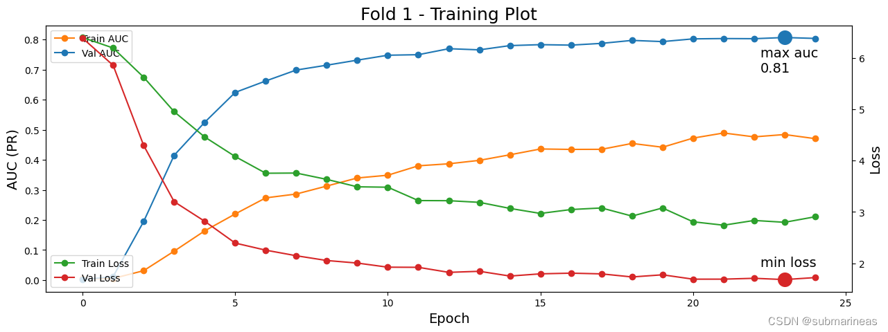
if CFG.training_plot:plot_history(history)

跑完大致输出可视化训练曲线为：

在这里插入图片描述
最后再进行训练，基本跟预训练的代码基本一致，就不再展开。但我遇到比较奇葩的事情是上述代码在Google的TPU下是没有什么问题的，即TPU v3，但我本地环境的GPU跑不过，可能是云环境下tensorflow是最新适配cuda 11.8的，而我在用cuda 11.2，所以我退了两个版本，错误如下，此处Mark一下：

在这里插入图片描述

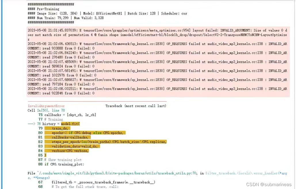
这里也算是踩坑的开始，我发现tensorflow报错一次性不是报一个，而是三四个，在issue中逛了一圈，啥也没看懂，到目前还没解决吧，于是换了个方案。

4. 优化方案 📈📊👩‍💻

关于优化，我做了比较多的尝试，比如说上述中我发现在本地跑不了预训练权重，于是退而求其次，直接拿着作者用8块TPU v3 做的权重进行后续的train，即预训练是TPU，训练是GPU，但我发现由于预训练的最高分数为0.81，我后续无论怎样调节参数，也很难超过该score了，很显然，0.81不是这个预训练的尽头，但kaggle平台上很难跑起这个数据集，后来我是将efficientnetB1换成了B0，才得到kaggle上单卡的pretrain_model，不过那样收效甚微，不知道哪里有问题，做了两次后停了，现在想想，其实是可以做一下消融实验的，最后是没做了，时间不够，以下是我的一些其它尝试。

4.1 微小提分点合集 🎭

本节中方法肯定是很多的，调参就不必说了，赛题的各种参数一堆，想调有机器可以调到天荒地老，不过我就前期跑了几次，中途发生了一些工作变动，导致没a100的机器跑了，后来换rtx 5000 * 2 搭好环境，把batch_size 改为 8，结果机器直接内存爆炸，赶紧重启保机器，之后虽然用非常规方式零零散散训练了几次，但就比较盲目，切私榜后发现还不如最开始的，现在想想，还是代码没写对。

4.1.1 data augment or TTA 🌈

在推理时，同样可以做TTA：

@tf.function(jit_compile=True)
def Audio2Spec(audio, spec_shape = CFG.img_size, sr=CFG.sample_rate, nfft=CFG.nfft, window=CFG.window, fmin=CFG.fmin, fmax=CFG.fmax, return_img=True):spec_height = spec_shape[0]spec_width = spec_shape[1]hop_length = tf.cast(CFG.hop_length, tf.int32) # sample rate * duration / spec width - 1 == 627spec = tfio.audio.spectrogram(audio, nfft=nfft, window=window, stride=hop_length)mel_spec = tfio.audio.melscale(spec, rate=sr, mels=spec_height, fmin=fmin, fmax=fmax)db_mel_spec = tfio.audio.dbscale(mel_spec, top_db=80)db_mel_spec = tf.linalg.matrix_transpose(db_mel_spec) # to keep it (batch, mel, time)return db_mel_spec@tf.function(jit_compile=True)
def Spec2Img(spec):spec = tf.tile(spec[..., tf.newaxis], [1, 1, 1, 3])return spec# Load audio from file and create audio frames, each recording will be a batch input
audio = load_audio(filepath)
chunks = MakeFrame(audio)#     # If not submitting, only use the first three frames for speed
#     if not SUBMIT:
#         chunks = chunks[:3]# Convert audio frames to spectrograms + rgb image using a vectorized function 
specs = Audio2Spec(chunks)
specs = Spec2Img(specs)

如上所示，这里可以在读出音频后，加上Audio2Spec 和 Spec2Img 这两步进行增强，在我实际测试中，有几个千分位的提升，但具体不清楚，因为我最后没用该方案。

4.1.2 addition data 📁

鸟类叫声的数据太多了，光是kaggle上并不仅仅就那么点，如果机器卡多，那还能增加更多dataset作为pretrain，但增加的dataset还是需要筛选一遍，比如我上面用的filter_data 和 upsample_data 两个函数针对极度不平衡状态下的补齐，当然也能直接剔除，我大概看了下目前base的预训练数据就已经130G，太大了，适当裁剪可能会有奇效，比如这次leaderboard 第一的就是选择了裁剪。以10为界限，删除了很多data小于10的类别。

4.1.3 调整threhold 🪄

这个东西在本赛题中其实作用不大，因为是264类物种的多分类，不过我后来没机器train，量化又遇到很多bug，最终还是采用了该方案，然后把我坑炸，LB切换的时候，给我掉了16名，不该玩这个的，但确确实实，它能在公榜上上分，原理就是下面这段代码：

for i in range(len(preds)):for j in range(len(preds[i])):if preds[i][j] > 0.0001: # arbitrary valuepasselse:preds[i][j] = 0.0            count = preds[i].sum()for j in range(len(preds[i])):preds[i][j] /= count # dividing by the sum re-normalises the predictions to 1

我最后交上去的就是启动了这个，两个threhold设置的是0.985和0.0015，公榜提升三个千分位，私榜掉了四个千分位，一切都是贪婪惹的祸。其实前排有个对此做了回复：

Why would you normalize the predictions per time window. Multiple birds can occur in one window, so it’s a multi-label problem.

只能说从40多名一路掉，没啥能commit，就玩这个了，emmm。。。

4.2 models ensemble ♻️

一般来讲，模型集成就是所提供的model分别做一次inference，然后可以求权值平均，voting或者stacking，但本题有点出入，如果直接集成，两个还好，三个不管什么模型都会timeout，限制了CPU推理两小时，所以还需要加点东西。

# Load all the models in memory to speed up
CKPTS = [tf.keras.models.load_model(x, compile=False) for x in tqdm(CKPT_PATHS, desc="Loading ckpts ")]
# Num of ckpt to use
NUM_CKPTS = 2def process_file(filepath):# Extract the filename without the extensionfilename = filepath.split('/')[-1].replace('.ogg','')# Load audio from file and create audio frames, each recording will be a batch inputaudio = load_audio(filepath)chunks = MakeFrame(audio)#     specs = Audio2Spec(chunks)
#     specs = Spec2Img(specs)# Predict bird species for all frames in a recording using all trained modelschunk_preds = np.zeros(shape=(len(chunks), 264), dtype=np.float32)for model in CKPTS[:NUM_CKPTS]:# Get the model's predictions for the current audio framesrec_preds = model(chunks, training=False).numpy()# Ensemble all prediction with averagechunk_preds += rec_preds/len(CKPTS)# Create a ID for each frame in a recording using the filename and frame numberrec_ids = [f'{filename}_{(frame_id+1)*5}' for frame_id in range(len(chunks))]return rec_ids, chunk_predsstart = time.time()
with concurrent.futures.ThreadPoolExecutor(max_workers=4) as executor:results = list(executor.map(process_file, test_df.filepath.tolist()))
print(f"With concurrent ThreadPoolExecutor, time cost reduced to {time.time()-start} for processing 15 audios")

我这里使用了两个模型做ensemble，前面都是常规操作，主要看最后四行，这里启用了四个线程去加速整个推理过程，那为什么启用四个呢？因为kaggle的notebook就只有两个CPU核心，worker设置再多，那跟四个的时间是一样的，这里我改写了几次，最开始还有两种，为：

results = Parallel(n_jobs=os.cpu_count())(delayed(process_file)(filepath) for filepath in tqdm(test_df.filepath.tolist(), 'test ')
)# Process the files in parallel
with concurrent.futures.ProcessPoolExecutor(max_workers=4) as executor:results = list(executor.map(process_file, test_df.filepath.tolist()))
print(f"With concurrent ThreadPoolExecutor, time cost reduced to {time.time()-start} for processing 15 audios")

第一种在pytorch中是可以的，但我这里带入tensorflow就不行了，原因是我的model最开始几层是用tensorflow_extra构建的，它并不支持并行化，当时直接给我干懵逼了，后来换了下面那一种，发现在kaggle平台上会卡住，最终才回到线程。

4.3 Quantization ⏰

我最后一礼拜，基本上都在研究如何量化，但很可惜，量化失败:(，不然我预估银牌肯定是保底的，因为我的最终方案就俩模型，前排都7个了，差距太大了，我现在回过头来，发现还是不该选用tensorflow作为baseline，根本没有留出太多可操作性，也可能是我懂得太少，没有探索到其中奥妙，这里就以我的经验，以及成功案例来总结。

一般作为pytorch，是有两种load方式，直接load是通用格式，而还有一种jit.load是用于加载 JIT 编译的模型，比如说第四名的方案：

models_ensemble = []
model1 = torch.jit.load(os.path.join(f"/kaggle/input/birdclef2023-4th-models/exp105_eca_nfnet_l0/", f"fold_0_model_jit_bs4.pt"))
model1.eval()
models_ensemble.append(model1)
model2 = torch.jit.load(os.path.join(f"/kaggle/input/birdclef2023-4th-models/exp106_eca_nfnet_l0/", f"fold_3_model_jit_bs4.pt"))
model2.eval()
models_ensemble.append(model2)
model3 = torch.jit.load(os.path.join(f"/kaggle/input/birdclef2023-4th-models/exp107_eca_nfnet_l0/", f"fold_4_model_jit_bs4.pt"))
model3.eval()
models_ensemble.append(model3)
model4 = torch.jit.load(os.path.join(f"/kaggle/input/birdclef2023-4th-models/exp108_eca_nfnet_l0/", f"fold_2_model_jit_bs4.pt"))
model4.eval()
models_ensemble.append(model4)

但tensorflow没有，因为它用的是不同的编译和执行方式。所以这里我就考虑了一手转为TFlite模型，正好我上场手势识别的比赛就是提交的tflite，即：

converter = tf.lite.TFLiteConverter.from_keras_model(model)
tflite_model = converter.convert()with open('model.tflite', 'wb') as f:f.write(tflite_model)

但最终效果不好，损失精度有点多，不知道是不是我这tensorflow的扩展依赖包问题，推理时间快了多少我也忘了，当时感觉太玄而又玄，就没试了。

然后过了两天在discussion上看到一个这样的方案：

params = list(model.parameters())
print('the length of parameters is', len(params))
for i in range(len(params)):params[i].data = torch.round(params[i].data*10**4) / 10**4

对模型精度进行四舍五入，我根据上面意思改写出了tensorflow的版本，为：

params = CKPTS[0].trainable_variables
print('the length of parameters is', len(params))for i in range(len(params)):params[i].assign(tf.round(params[i]*10**4) / 10**4)# 保存模型
CKPTS[0].save('/kaggle/working/update_fold_10.h5')

在我的测试下，速度确实有所提升，tensorflow平均一个模型降了4s多，总共就从三模型推理集成为73s降到了61s，按理说这就已经够了，我做了一个benchmark，就是浪费了5次提交，测出本地我上面模型推理时间必须在64s以内，可奇怪就奇怪在，我本地调试时间已经在64s内了，但只要commit，时间又回去了，不知道是哪里的问题，后续又用pytorch的模型试了下，加jit与精度舍入，从19s降到10s左右，整整两倍的提升，不过没提交，不然可以排除一个干扰选项。

再后来就去研究pytorch的 QUANTIZATION ，以及tensorflow_model_optimization 这个包，然后，比赛结束。

4.3.1 openvino 优化模型 📈

赛后看到前排方案里用openvino，恍然大悟，咋就没想到捏，忘了Intel这种专门做CPU加速的公司了，太可惜了。其转化也非常简单，为：

input_names = [ "x",'tta_delta' ]
output_names = [ "clipwise_output" ]torch.onnx.export(model, input_sed, "sed64.onnx", verbose=False, input_names=input_names, output_names=output_names)!mo --input_model sed64.onnximport openvino.runtime as ov
core = ov.Core()
openvino_model = core.read_model(model='sed64.xml')
compiled_model = core.compile_model(openvino_model, device_name="CPU")
infer_request = compiled_model.create_infer_request()

这里经过测试，推理时间又快了接近2倍。

5. 前排方案 📈📊🦉

5.1——1th：Correct Data is All You Need 🏆

不愧是第一名，开篇直抒胸臆：

If You Only Knew the Power of A100s GPUs

作者说做了 294 experiments，我如果只算train的，可能不到10次。。。

然后看得出，add了非常多的dataset，model选用了3个声音事件检测(SED)模型，为：

eca_nfnet_l0 (2 stages training; Start LR 1e-3)
convnext_small_fb_in22k_ft_in1k_384 (2 stages training; Start LR 1e-4)
convnextv2_tiny_fcmae_ft_in22k_in1k_384 (1 stage training; Start LR 1e-4)

数据增强方案为：

Mixup : Simply OR Mixup with Prob = 0.5
BackgroundNoise with Zenodo nocall
RandomFiltering - a custom augmentation: in simple terms, it’s a simplified random Equalizer
Spec Aug：
- Freq：
  - Max length: 10
  - Max lines: 3
  - Probability: 0.3
- Time：
  - Max length: 20
  - Max lines: 3
  - Probability: 0.3

从以上来看，从模型到参数设置确实与我不太一样，我都是用的主流数据，后续也改动很少。

这里还有两个trick，为：

Using temperature mean： pred = (pred**2).mean(axis=0) ** 0.5
Using Attention SED probs * 0.75 + Max Timewise probs * 0.25

能看懂，但不太清楚对应的具体业务背景是什么，可能还需要具体的对照实验才行。

5.2——2th：2nd place solution: SED + CNN with 7 models ensemble 🥈

第二名方案采用了openvino 基本将模型堆到了极致，框架使用了SED architecture，七个模型的backbone为：

tf_efficientnetv2_s_in21k
seresnext26t_32x4d
tf_efficientnet_b3_ns
tf_efficientnetv2_s_in21k
resnet34d
tf_efficientnet_b3_ns
tf_efficientnet_b0_ns

然后加入了一堆数据增强，这里就不列举了，看标的竟然有十几种。。。那训练集相当于扩增了接近十倍，因为也做了预训练，最终为啥能推理起来，应该是做了CV strategy，为For each validation sample - slice the first 60 seconds to pieces -> predict each piece -> max(sample_predictions, dim=pieces). 套路太强了。

5.3——4th：Knowledge Distillation Is All You Need 🏅

排除与前面方案一致的trick，第四名做了一组很有意思的实验：

MelSpectrogram (sample_rate: 32000, mel_bins: 128, fmin: 20, fmax: 16000, window_size: 2048, hop_size: 512, top_db=80.0, NormalizeMelSpec) following this solution.
- Public: 0.8312, Private: 0.74424
Balanced sampling with the above settings.
- Public: 0.83106, Private: 0.74406
PCEN (sample_rate: 32000, mel_bins: 128, fmin: 20, fmax: 16000, window_size: 2048, hop_size: 512).
- Public: 0.83005, Private: 0.74134
MelSpectrogram (sample_rate: 32000, mel_bins: 64, fmin: 50, fmax: 14000, window_size: 1024, hop_size: 320).
- Public: 0.83014, Private: 0.74201

以及一些train的trick：

Using 5 StratifiedKFold. Only 1 fold did not cover all classes, so the remaining 4 were used for training.
The evaluation metric is padded_cmap1. The best results were the same with padded_cmap5 in most cases.
Use primary_label only
no-call is represented by all 0
loss: 0.1 * BCEWithLogitsLoss (primary_label) + 0.9 * KLDivLoss (from Kaggle model)
- Softmax temperature=20 was best (tried 5, 10, 20, 30).
I used randomly sampled 20-sec clips for training. Audio that is less than 20 sec is repeated.
epoch = 400 (Most models converge at 100-300)
early stopping(pretraining=10, training=20)
Optimizer: AdamW (lr: pretraining=5e-4, training=2.5e-4, wd: 1e-6)
CosineLRScheduler(t_initial=10, warmup_t=1, cycle_limit=40, cycle_decay=1.0, lr_min=1e-7, t_in_epochs=True,)
mixup p = 1.0

5.4—— 6th：BirdNET embedding + CNN 🏅

第六名的方案可以用一张流程图进行表示，为：

在这里插入图片描述

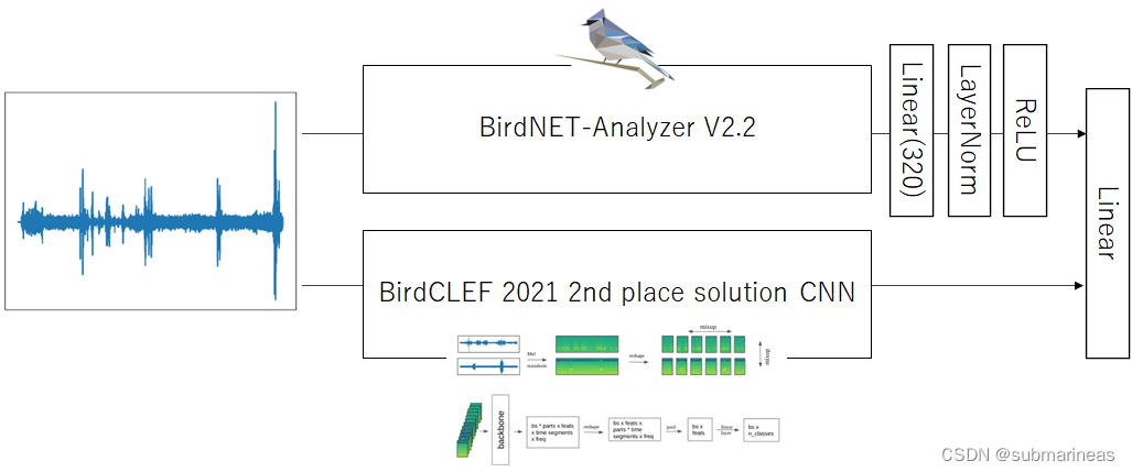
这里不再详述，附上这种框架下大致的一个分数为：

name	Private Score	Public Score
BirdCLEF 2021 2nd place solution CNN (with BirdCLEF 2021 + BirdCLEF 2022 pretrain)	0.71	0.80
BirdCLEF 2021 2nd place solution CNN + Augmentation + BirdNET embedding	0.74	0.82
BirdCLEF 2021 2nd place solution CNN + Augmentation + BirdNET embedding + Oversampling + Ensembling	0.75	0.83