Lib01 多变量线性回归
依旧是房价预测,但这次引入了多个变量,不仅仅只有房屋面积影响着房价,依旧尝试使用梯度下降算法找到最优的【w,b】,并且习惯使用向量点乘运算提高效率
import copy, math
import numpy as np
import matplotlib.pyplot as plt
plt.style.use('./deeplearning.mplstyle')
np.set_printoptions(precision=2)  #保留小数点后两位
X_train = np.array([[2104, 5, 1, 45], [1416, 3, 2, 40], [852, 2, 1, 35]])
y_train = np.array([460, 232, 178])
print(X_train)
print(y_train)只有三组数据的训练集,全转成向量存储,方便点乘运算
X_train中包含了三栋房子,即三个向量,每个向量都包含了四个特征值:面积,房间数,层数,房屋已使用年数
y_train中则为三栋房子的价格
b_init = 785.1811367994083
w_init = np.array([ 0.39133535, 18.75376741, -53.36032453, -26.42131618])
作为练习,w,b的值初始化为了接近最优值的数值,方便更快地找到
def compute_gradient(X,y,w,b):m,n = X.shape #行给m,列给ndj_dw = np.zeros((n,))dj_db = 0.0for i in range(m):err = (np.dot(X[i],w)+b)-y[i] #np.dot(X[i],w)表示所有特征与w相乘后得到新的向量for j in range(n):dj_dw[j] += err*X[i,j] #X[i,j]:第i组数据第j个特征值dj_db += errdj_dw /= mdj_db /= mreturn dj_dw,dj_db计算偏导数的函数,如果忘记推导过程可以看看上一节的文章
def compute_cost(X,y,w,b):m = X.shape[0] #一行有几个特征值 cost = 0.0 for i in range(m):err = np.dot(X[i],w)+b-y[i]cost += err**2return cost/(2.0*m)代价函数J的计算
def gradient_descent(X, y, w_in, b_in, cost_function, gradient_function, alpha, num_iters): J_history = [] #记录每对[w,b]的cost值w = copy.deepcopy(w_in)b = b_infor i in range(num_iters):dj_dw,dj_db = gradient_function(X,y,w,b)w = w - alpha*dj_dwb = b - alpha*dj_dbif i<10000:J_history.append(cost_function(X,y,w,b))if i% math.ceil(num_iters / 10) == 0:print(f"Iteration {i:4d}: Cost {J_history[-1]:8.2f} ")return w,b,J_history梯度下降算法的实现
initial_w = np.zeros_like(w_init)
initial_b = 0.0
iterations = 1000
alpha = 5.0e-7
w_final,b_final,J_hist = gradient_descent(X_train,y_train,initial_w,initial_b,compute_cost,compute_gradient,alpha,iterations)
print(f"最优的w值为{w_final:}\n最优的b值为{b_final:0.2f}")
m = X_train.shape[0]
for i in range(m):print(f"预测值:{np.dot(w_final,X_train[i])+b_final:0.2f} 实际值:{y_train[i]}" )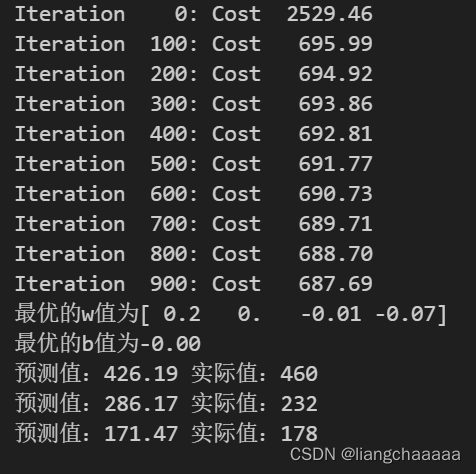
迭代求解w,b并进行预测
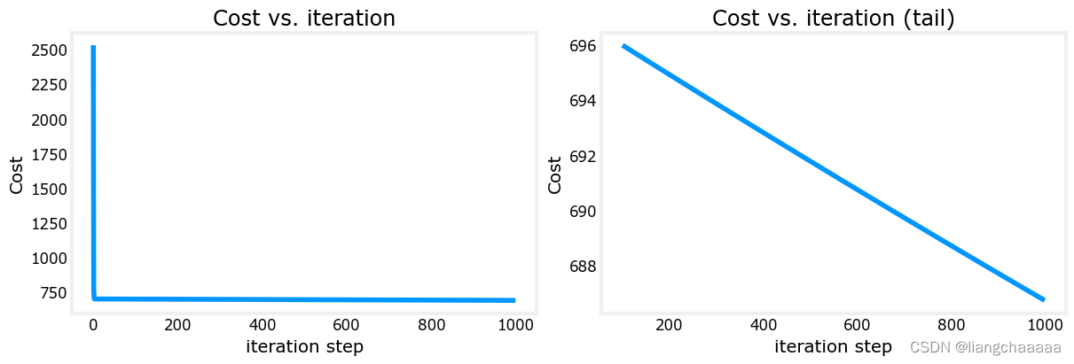
数据的可视化
完整版代码
import copy, math
import numpy as np
import matplotlib.pyplot as plt
#plt.style.use('./deeplearning.mplstyle')
np.set_printoptions(precision=2)  #保留小数点后两位X_train = np.array([[2104, 5, 1, 45], [1416, 3, 2, 40], [852, 2, 1, 35]])
y_train = np.array([460, 232, 178])
b_init = 785.1811367994083
w_init = np.array([ 0.39133535, 18.75376741, -53.36032453, -26.42131618])def compute_gradient(X,y,w,b):m,n = X.shape #行给m,列给ndj_dw = np.zeros((n,))dj_db = 0.0for i in range(m):err = (np.dot(X[i],w)+b)-y[i] #np.dot(X[i],w)表示所有特征与w相乘后得到新的向量for j in range(n):dj_dw[j] += err*X[i,j] #X[i,j]:第i组数据第j个特征值dj_db += errdj_dw /= mdj_db /= mreturn dj_dw,dj_dbdef compute_cost(X,y,w,b):m = X.shape[0] #一行有几个特征值 cost = 0.0  for i in range(m):err = np.dot(X[i],w)+b-y[i]cost += err**2return cost/(2.0*m)def predict(x,w,b):y = np.dot(x,w)+breturn ydef gradient_descent(X, y, w_in, b_in, cost_function, gradient_function, alpha, num_iters): J_history = [] #记录每对[w,b]的cost值w = copy.deepcopy(w_in)b = b_infor i in range(num_iters):dj_dw,dj_db = gradient_function(X,y,w,b)w = w - alpha*dj_dwb = b - alpha*dj_dbif i<10000:J_history.append(cost_function(X,y,w,b))if i% math.ceil(num_iters / 10) == 0:print(f"Iteration {i:4d}: Cost {J_history[-1]:8.2f}   ")return w,b,J_historyinitial_w = np.zeros_like(w_init)
initial_b = 0.0
iterations = 1000
alpha = 5.0e-7
w_final,b_final,J_hist = gradient_descent(X_train,y_train,initial_w,initial_b,compute_cost,compute_gradient,alpha,iterations)
print(f"最优的w值为{w_final:}\n最优的b值为{b_final:0.2f}")
m = X_train.shape[0]
for i in range(m):print(f"预测值:{np.dot(w_final,X_train[i])+b_final:0.2f} 实际值:{y_train[i]}" )# plot cost versus iteration
fig, (ax1, ax2) = plt.subplots(1, 2, constrained_layout=True, figsize=(12, 4))
ax1.plot(J_hist)
ax2.plot(100 + np.arange(len(J_hist[100:])), J_hist[100:])
ax1.set_title("Cost vs. iteration");  ax2.set_title("Cost vs. iteration (tail)")
ax1.set_ylabel('Cost')             ;  ax2.set_ylabel('Cost')
ax1.set_xlabel('iteration step')   ;  ax2.set_xlabel('iteration step')
plt.show()
Lib02 特征缩放、学习速率选择
import numpy as np
np.set_printoptions(precision=2)
import matplotlib.pyplot as plt
dlblue = '#0096ff'; dlorange = '#FF9300'; dldarkred='#C00000'; dlmagenta='#FF40FF'; dlpurple='#7030A0';
plt.style.use('./deeplearning.mplstyle')
from lab_utils_multi import  load_house_data, compute_cost, run_gradient_descent
from lab_utils_multi import  norm_plot, plt_contour_multi, plt_equal_scale, plot_cost_i_w
这里需要把lab_utils_multi.py文件放在和程序相同目录下,源文件放在了文章的开头和末尾
# load the dataset
X_train, y_train = load_house_data()
X_features = ['size(sqft)','bedrooms','floors','age']
上图为load_house_data函数原型,导入官方房价预测训练集,delimiter=','以逗号为分隔符,skiprows=1跳过文件的第一行(即文件头)
fig,ax=plt.subplots(1, 4, figsize=(12, 3), sharey=True)
for i in range(len(ax)):ax[i].scatter(X_train[:,i],y_train)ax[i].set_xlabel(X_features[i])
ax[0].set_ylabel("Price (1000's)")
plt.show()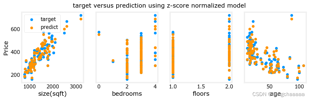
数据集可视化,fig,ax=plt.subplots(1, 4, figsize=(12, 3), sharey=True),创建了一个大小为12x3的图形窗口,其中包含一行四列子图。每个子图可以通过在1行和4列中指定位置的ax参数来访问。这些子图共享一个y轴,通过设置sharey=True来实现。
学习速率α的尝试
#set alpha to 9.9e-7
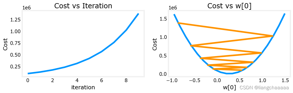
_, _, hist = run_gradient_descent(X_train, y_train, 10, alpha = 9.9e-7)
plot_cost_i_w(X_train, y_train, hist)梯度下降的算法实现与之前大体一致,我们把学习速率设置为了9.9e-7,并作图观察梯度下降的过程。看图得知。每次迭代w[0]改变幅度过大超出了期望的值范围,导致cost最终在不断变大而非接近最小值即最优解。但这张图只显示了w0,这并不是一幅完全准确的图画,因为每次有4个参数被修改,而不是只有一个,其他参数固定在良性值。
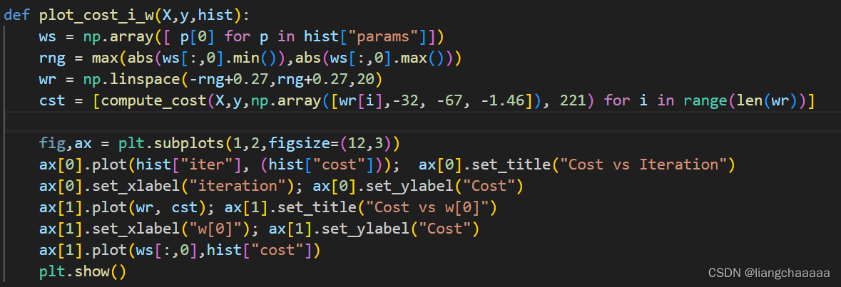
上图为plot_cost_i_w函数原型,如果自己手动改变查看w1,w2等其他参数的迭代过程图,可以在 lab_utils_multi.py文件的源码中修改compute_cost函数传入参数的NDArray数组
_,_,hist = run_gradient_descent(X_train, y_train, 10, alpha = 9e-7)
plot_cost_i_w(X_train, y_train, hist)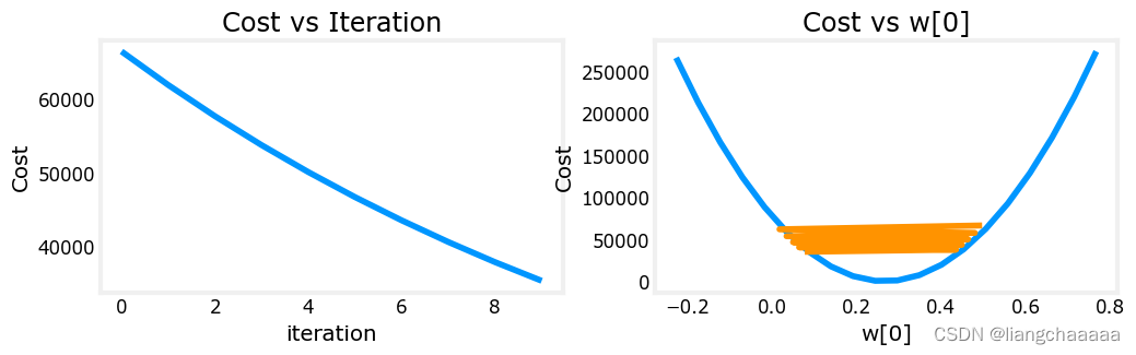
学习速率稍微改小一点,改成9e-7时,迭代过程如图,迭代的过程跳动幅度也很大,但是cost是在不断下降的,最终是会收敛的
特征值缩放
先说说为什么对特征值进行缩放。如下图,房间数和屋子面积在数值上相差较大,相差约为几百倍,如果严格按照数值大小作为坐标轴尺度,发现所有的点几乎都“贴”在x轴上,contour等高线图上是一个很扁的椭圆而非圆。那么,在梯度下降的时候,就有可能跨过或忽略了最小值,导致一直来回震荡而无法收敛的情况。所以我们需要进行合适的缩放,来确保算法能找到正确的解。

Z-Score标准化(特征值缩放的一种方法)
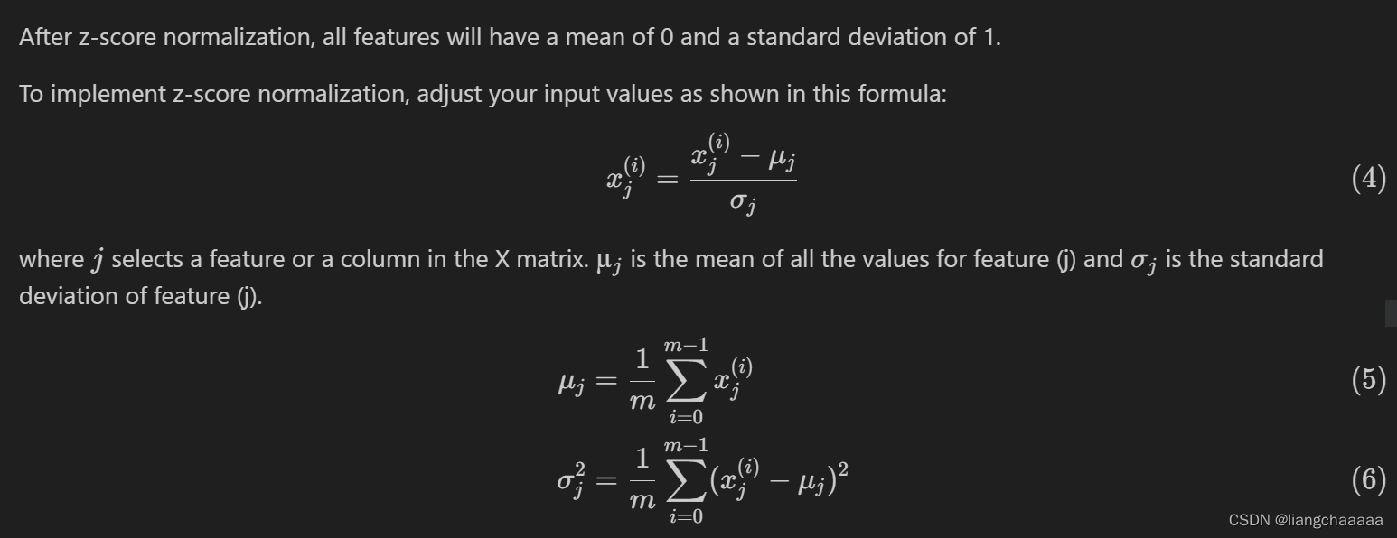
:该特征值的平均值
:该特征值的标准差
def zscore_normalize_features(X):#X是一个有m组数组,每组数据有n个特征值的向量mu = np.mean(X, axis=0) #平均值 sigma = np.std(X, axis=0) #标准差 X_norm = (X - mu) / sigma #sigma和mu均为n维向量(因为有n个特征值)#X_norm为标准化后的向量,mu为每个特征值的平均值的向量,sigma为标准差return (X_norm, mu, sigma)进行标准化之前

X_norm, X_mu, X_sigma = zscore_normalize_features(X_train)进行标准化之后
Lib02 完整版代码
注意数据集和lab_utils_multi.py也要放在同一目录下
import numpy as np
np.set_printoptions(precision=2)
import matplotlib.pyplot as plt
dlblue = '#0096ff'; dlorange = '#FF9300'; dldarkred='#C00000'; dlmagenta='#FF40FF'; dlpurple='#7030A0';
#plt.style.use('./deeplearning.mplstyle')
from lab_utils_multi import load_house_data, compute_cost, run_gradient_descent
from lab_utils_multi import norm_plot, plt_contour_multi, plt_equal_scale, plot_cost_i_w# load the dataset
X_train, y_train = load_house_data()
X_features = ['size(sqft)','bedrooms','floors','age']fig,ax=plt.subplots(1, 4, figsize=(12, 3), sharey=True)
for i in range(len(ax)):ax[i].scatter(X_train[:,i],y_train)ax[i].set_xlabel(X_features[i])
ax[0].set_ylabel("Price (1000's)")
plt.show()#set alpha to 9.9e-7
_, _, hist = run_gradient_descent(X_train, y_train, 10, alpha = 9.9e-7)
plot_cost_i_w(X_train, y_train, hist)#set alpha to 9e-7
_,_,hist = run_gradient_descent(X_train, y_train, 10, alpha = 9e-7)
plot_cost_i_w(X_train, y_train, hist)#set alpha to 1e-7
_,_,hist = run_gradient_descent(X_train, y_train, 10, alpha = 1e-7)
plot_cost_i_w(X_train, y_train, hist)def zscore_normalize_features(X):"""computes X, zcore normalized by columnArgs:X (ndarray): Shape (m,n) input data, m examples, n featuresReturns:X_norm (ndarray): Shape (m,n) input normalized by columnmu (ndarray): Shape (n,) mean of each featuresigma (ndarray): Shape (n,) standard deviation of each feature"""# find the mean of each column/featuremu = np.mean(X, axis=0) # mu will have shape (n,)# find the standard deviation of each column/featuresigma = np.std(X, axis=0) # sigma will have shape (n,)# element-wise, subtract mu for that column from each example, divide by std for that columnX_norm = (X - mu) / sigma return (X_norm, mu, sigma)mu = np.mean(X_train,axis=0)
sigma = np.std(X_train,axis=0)
X_mean = (X_train - mu)
X_norm = (X_train - mu)/sigma fig,ax=plt.subplots(1, 3, figsize=(12, 3))
ax[0].scatter(X_train[:,0], X_train[:,3])
ax[0].set_xlabel(X_features[0]); ax[0].set_ylabel(X_features[3]);
ax[0].set_title("unnormalized")
ax[0].axis('equal')ax[1].scatter(X_mean[:,0], X_mean[:,3])
ax[1].set_xlabel(X_features[0]); ax[0].set_ylabel(X_features[3]);
ax[1].set_title(r"X - $\mu$")
ax[1].axis('equal')ax[2].scatter(X_norm[:,0], X_norm[:,3])
ax[2].set_xlabel(X_features[0]); ax[0].set_ylabel(X_features[3]);
ax[2].set_title(r"Z-score normalized")
ax[2].axis('equal')
plt.tight_layout(rect=[0, 0.03, 1, 0.95])
fig.suptitle("distribution of features before, during, after normalization")
plt.show()# normalize the original features
X_norm, X_mu, X_sigma = zscore_normalize_features(X_train)
print(f"X_mu = {X_mu}, \nX_sigma = {X_sigma}")
print(f"Peak to Peak range by column in Raw X:{np.ptp(X_train,axis=0)}")
print(f"Peak to Peak range by column in Normalized X:{np.ptp(X_norm,axis=0)}")fig,ax=plt.subplots(1, 4, figsize=(12, 3))
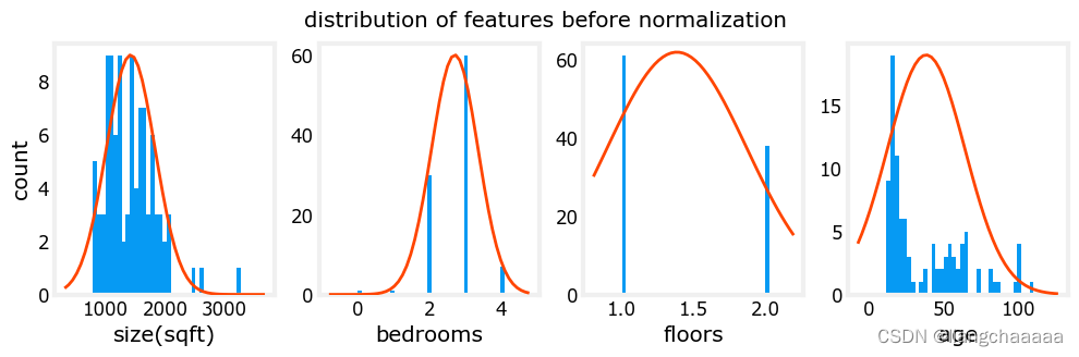
for i in range(len(ax)):norm_plot(ax[i],X_train[:,i],)ax[i].set_xlabel(X_features[i])
ax[0].set_ylabel("count");
fig.suptitle("distribution of features before normalization")
plt.show()
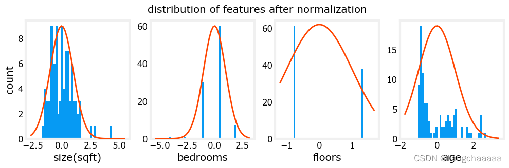
X_norm, X_mu, X_sigma = zscore_normalize_features(X_train)
fig,ax=plt.subplots(1,4,figsize=(12,3))
for i in range(len(ax)):norm_plot(ax[i],X_norm[:,i],)ax[i].set_xlabel(X_features[i])
ax[0].set_ylabel("count");
fig.suptitle(f"distribution of features after normalization")plt.show()Lib03 多项式回归
实际回归中,数据不一定都是线性的,让我们尝试用我们目前所知的知识来拟合一条非线性曲线。
# create target data
x = np.arange(0, 20, 1) #包含数字 0 到 19
y = 1 + x**2
X = x.reshape(-1, 1)  #(20,1)
#-1参数的作用是让 NumPy 自动计算该轴长度,在本例中由原始的长度为 20 推断为自动适应后的长度为 20 行;
#1参数表示将x重新组织为一个一列多行的数组。model_w,model_b = run_gradient_descent_feng(X,y,iterations=1000, alpha = 1e-2)plt.scatter(x, y, marker='x', c='r', label="Actual Value"); plt.title("no feature engineering")
plt.plot(x,X@model_w + model_b, label="Predicted Value");  plt.xlabel("X"); plt.ylabel("y"); plt.legend(); plt.show()
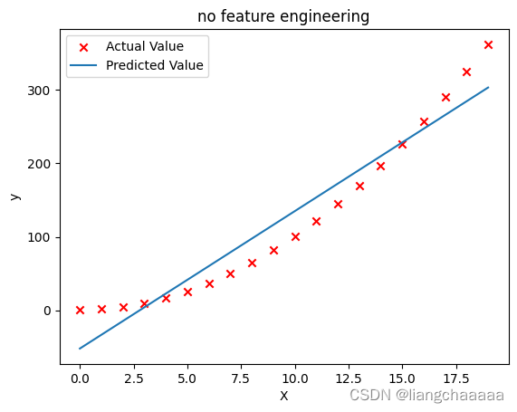
显然,我绘制的是二次函数,一元多项式回归的拟合效果当然不好
# create target data
x = np.arange(0, 20, 1)
y = 1 + x**2# Engineer features
X = x**2      #<-- added engineered feature
#X = np.c_[x, x**2, x**3] 你也可以这么加,变成一个多项式X = X.reshape(-1, 1)  #X should be a 2-D Matrix
model_w,model_b = run_gradient_descent_feng(X, y, iterations=10000, alpha = 1e-5)plt.scatter(x, y, marker='x', c='r', label="Actual Value"); plt.title("Added x**2 feature")
plt.plot(x, np.dot(X,model_w) + model_b, label="Predicted Value"); plt.xlabel("x"); plt.ylabel("y"); plt.legend(); plt.show()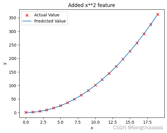
特征工程换成二元多项式可以很好的拟合数据
x = np.arange(0,20,1)
y = np.cos(x/2)X = np.c_[x, x**2, x**3,x**4, x**5, x**6, x**7, x**8, x**9, x**10, x**11, x**12, x**13]
X = zscore_normalize_features(X) model_w,model_b = run_gradient_descent_feng(X, y, iterations=1000000, alpha = 1e-1)plt.scatter(x, y, marker='x', c='r', label="Actual Value"); plt.title("Normalized x x**2, x**3 feature")
plt.plot(x,X@model_w + model_b, label="Predicted Value"); plt.xlabel("x"); plt.ylabel("y"); plt.legend(); plt.show()
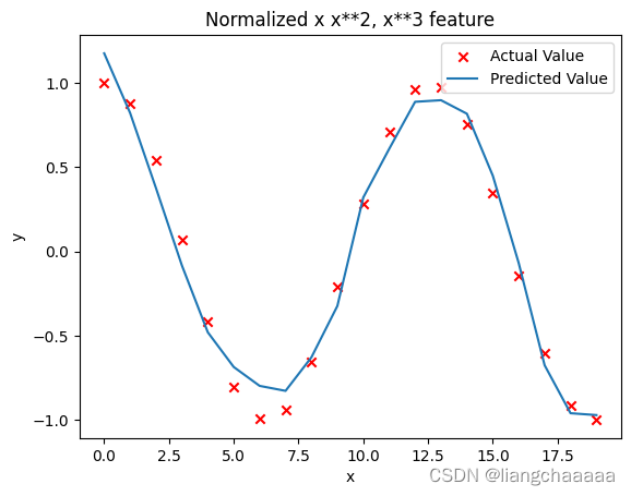
遇到复杂的函数,特征工程就不是那么好建立了,而在sklearn中有封装好的方法(
sklearn.preprocessing.PolynomialFeatures)帮助我们建立特征工程,这里先开个头引入多项式回归,之后探讨一下热门的sklearn库中函数
lab_utils_multi.py源代码
import numpy as np
import copy
import math
from scipy.stats import norm
import matplotlib.pyplot as plt
from mpl_toolkits.mplot3d import axes3d
from matplotlib.ticker import MaxNLocator
dlblue = '#0096ff'; dlorange = '#FF9300'; dldarkred='#C00000'; dlmagenta='#FF40FF'; dlpurple='#7030A0';
plt.style.use('./deeplearning.mplstyle')def load_data_multi():data = np.loadtxt("data/ex1data2.txt", delimiter=',')X = data[:,:2]y = data[:,2]return X, y##########################################################
# Plotting Routines
##########################################################def plt_house_x(X, y,f_wb=None, ax=None):''' plot house with aXis '''if not ax:fig, ax = plt.subplots(1,1)ax.scatter(X, y, marker='x', c='r', label="Actual Value")ax.set_title("Housing Prices")ax.set_ylabel('Price (in 1000s of dollars)')ax.set_xlabel(f'Size (1000 sqft)')if f_wb is not None:ax.plot(X, f_wb,  c=dlblue, label="Our Prediction")ax.legend()def mk_cost_lines(x,y,w,b, ax):''' makes vertical cost lines'''cstr = "cost = (1/2m)*1000*("ctot = 0label = 'cost for point'for p in zip(x,y):f_wb_p = w*p[0]+bc_p = ((f_wb_p - p[1])**2)/2c_p_txt = c_p/1000ax.vlines(p[0], p[1],f_wb_p, lw=3, color=dlpurple, ls='dotted', label=label)label='' #just onecxy = [p[0], p[1] + (f_wb_p-p[1])/2]ax.annotate(f'{c_p_txt:0.0f}', xy=cxy, xycoords='data',color=dlpurple, xytext=(5, 0), textcoords='offset points')cstr += f"{c_p_txt:0.0f} +"ctot += c_pctot = ctot/(len(x))cstr = cstr[:-1] + f") = {ctot:0.0f}"ax.text(0.15,0.02,cstr, transform=ax.transAxes, color=dlpurple)def inbounds(a,b,xlim,ylim):xlow,xhigh = xlimylow,yhigh = ylimax, ay = abx, by = bif (ax > xlow and ax < xhigh) and (bx > xlow and bx < xhigh) \and (ay > ylow and ay < yhigh) and (by > ylow and by < yhigh):return(True)else:return(False)from mpl_toolkits.mplot3d import axes3d
def plt_contour_wgrad(x, y, hist, ax, w_range=[-100, 500, 5], b_range=[-500, 500, 5], contours = [0.1,50,1000,5000,10000,25000,50000], resolution=5, w_final=200, b_final=100,step=10 ):b0,w0 = np.meshgrid(np.arange(*b_range),np.arange(*w_range))z=np.zeros_like(b0)n,_ = w0.shapefor i in range(w0.shape[0]):for j in range(w0.shape[1]):z[i][j] = compute_cost(x, y, w0[i][j], b0[i][j] )CS = ax.contour(w0, b0, z, contours, linewidths=2,colors=[dlblue, dlorange, dldarkred, dlmagenta, dlpurple]) ax.clabel(CS, inline=1, fmt='%1.0f', fontsize=10)ax.set_xlabel("w");  ax.set_ylabel("b")ax.set_title('Contour plot of cost J(w,b), vs b,w with path of gradient descent')w = w_final; b=b_finalax.hlines(b, ax.get_xlim()[0],w, lw=2, color=dlpurple, ls='dotted')ax.vlines(w, ax.get_ylim()[0],b, lw=2, color=dlpurple, ls='dotted')base = hist[0]for point in hist[0::step]:edist = np.sqrt((base[0] - point[0])**2 + (base[1] - point[1])**2)if(edist > resolution or point==hist[-1]):if inbounds(point,base, ax.get_xlim(),ax.get_ylim()):plt.annotate('', xy=point, xytext=base,xycoords='data',arrowprops={'arrowstyle': '->', 'color': 'r', 'lw': 3},va='center', ha='center')base=pointreturn# plots p1 vs p2. Prange is an array of entries [min, max, steps]. In feature scaling lab.
def plt_contour_multi(x, y, w, b, ax, prange, p1, p2, title="", xlabel="", ylabel=""): contours = [1e2, 2e2,3e2,4e2, 5e2, 6e2, 7e2,8e2,1e3, 1.25e3,1.5e3, 1e4, 1e5, 1e6, 1e7]px,py = np.meshgrid(np.linspace(*(prange[p1])),np.linspace(*(prange[p2])))z=np.zeros_like(px)n,_ = px.shapefor i in range(px.shape[0]):for j in range(px.shape[1]):w_ij = wb_ij = bif p1 <= 3: w_ij[p1] = px[i,j]if p1 == 4: b_ij = px[i,j]if p2 <= 3: w_ij[p2] = py[i,j]if p2 == 4: b_ij = py[i,j]z[i][j] = compute_cost(x, y, w_ij, b_ij )CS = ax.contour(px, py, z, contours, linewidths=2,colors=[dlblue, dlorange, dldarkred, dlmagenta, dlpurple]) ax.clabel(CS, inline=1, fmt='%1.2e', fontsize=10)ax.set_xlabel(xlabel);  ax.set_ylabel(ylabel)ax.set_title(title, fontsize=14)def plt_equal_scale(X_train, X_norm, y_train):fig,ax = plt.subplots(1,2,figsize=(12,5))prange = [[ 0.238-0.045, 0.238+0.045,  50],[-25.77326319-0.045, -25.77326319+0.045, 50],[-50000, 0,      50],[-1500,  0,      50],[0, 200000, 50]]w_best = np.array([0.23844318, -25.77326319, -58.11084634,  -1.57727192])b_best = 235plt_contour_multi(X_train, y_train, w_best, b_best, ax[0], prange, 0, 1, title='Unnormalized, J(w,b), vs w[0],w[1]',xlabel= "w[0] (size(sqft))", ylabel="w[1] (# bedrooms)")#w_best = np.array([111.1972, -16.75480051, -28.51530411, -37.17305735])b_best = 376.949151515151prange = [[ 111-50, 111+50,   75],[-16.75-50,-16.75+50, 75],[-28.5-8, -28.5+8,  50],[-37.1-16,-37.1+16, 50],[376-150, 376+150, 50]]plt_contour_multi(X_norm, y_train, w_best, b_best, ax[1], prange, 0, 1, title='Normalized, J(w,b), vs w[0],w[1]',xlabel= "w[0] (normalized size(sqft))", ylabel="w[1] (normalized # bedrooms)")fig.suptitle("Cost contour with equal scale", fontsize=18)#plt.tight_layout(rect=(0,0,1.05,1.05))fig.tight_layout(rect=(0,0,1,0.95))plt.show()def plt_divergence(p_hist, J_hist, x_train,y_train):x=np.zeros(len(p_hist))y=np.zeros(len(p_hist))v=np.zeros(len(p_hist))for i in range(len(p_hist)):x[i] = p_hist[i][0]y[i] = p_hist[i][1]v[i] = J_hist[i]fig = plt.figure(figsize=(12,5))plt.subplots_adjust( wspace=0 )gs = fig.add_gridspec(1, 5)fig.suptitle(f"Cost escalates when learning rate is too large")#===============#  First subplot#===============ax = fig.add_subplot(gs[:2], )# Print w vs cost to see minimumfix_b = 100w_array = np.arange(-70000, 70000, 1000)cost = np.zeros_like(w_array)for i in range(len(w_array)):tmp_w = w_array[i]cost[i] = compute_cost(x_train, y_train, tmp_w, fix_b)ax.plot(w_array, cost)ax.plot(x,v, c=dlmagenta)ax.set_title("Cost vs w, b set to 100")ax.set_ylabel('Cost')ax.set_xlabel('w')ax.xaxis.set_major_locator(MaxNLocator(2)) #===============# Second Subplot#===============tmp_b,tmp_w = np.meshgrid(np.arange(-35000, 35000, 500),np.arange(-70000, 70000, 500))z=np.zeros_like(tmp_b)for i in range(tmp_w.shape[0]):for j in range(tmp_w.shape[1]):z[i][j] = compute_cost(x_train, y_train, tmp_w[i][j], tmp_b[i][j] )ax = fig.add_subplot(gs[2:], projection='3d')ax.plot_surface(tmp_w, tmp_b, z,  alpha=0.3, color=dlblue)ax.xaxis.set_major_locator(MaxNLocator(2)) ax.yaxis.set_major_locator(MaxNLocator(2)) ax.set_xlabel('w', fontsize=16)ax.set_ylabel('b', fontsize=16)ax.set_zlabel('\ncost', fontsize=16)plt.title('Cost vs (b, w)')# Customize the view angle ax.view_init(elev=20., azim=-65)ax.plot(x, y, v,c=dlmagenta)return# draw derivative line
# y = m*(x - x1) + y1
def add_line(dj_dx, x1, y1, d, ax):x = np.linspace(x1-d, x1+d,50)y = dj_dx*(x - x1) + y1ax.scatter(x1, y1, color=dlblue, s=50)ax.plot(x, y, '--', c=dldarkred,zorder=10, linewidth = 1)xoff = 30 if x1 == 200 else 10ax.annotate(r"$\frac{\partial J}{\partial w}$ =%d" % dj_dx, fontsize=14,xy=(x1, y1), xycoords='data',xytext=(xoff, 10), textcoords='offset points',arrowprops=dict(arrowstyle="->"),horizontalalignment='left', verticalalignment='top')def plt_gradients(x_train,y_train, f_compute_cost, f_compute_gradient):#===============#  First subplot#===============fig,ax = plt.subplots(1,2,figsize=(12,4))# Print w vs cost to see minimumfix_b = 100w_array = np.linspace(-100, 500, 50)w_array = np.linspace(0, 400, 50)cost = np.zeros_like(w_array)for i in range(len(w_array)):tmp_w = w_array[i]cost[i] = f_compute_cost(x_train, y_train, tmp_w, fix_b)ax[0].plot(w_array, cost,linewidth=1)ax[0].set_title("Cost vs w, with gradient; b set to 100")ax[0].set_ylabel('Cost')ax[0].set_xlabel('w')# plot lines for fixed b=100for tmp_w in [100,200,300]:fix_b = 100dj_dw,dj_db = f_compute_gradient(x_train, y_train, tmp_w, fix_b )j = f_compute_cost(x_train, y_train, tmp_w, fix_b)add_line(dj_dw, tmp_w, j, 30, ax[0])#===============# Second Subplot#===============tmp_b,tmp_w = np.meshgrid(np.linspace(-200, 200, 10), np.linspace(-100, 600, 10))U = np.zeros_like(tmp_w)V = np.zeros_like(tmp_b)for i in range(tmp_w.shape[0]):for j in range(tmp_w.shape[1]):U[i][j], V[i][j] = f_compute_gradient(x_train, y_train, tmp_w[i][j], tmp_b[i][j] )X = tmp_wY = tmp_bn=-2color_array = np.sqrt(((V-n)/2)**2 + ((U-n)/2)**2)ax[1].set_title('Gradient shown in quiver plot')Q = ax[1].quiver(X, Y, U, V, color_array, units='width', )qk = ax[1].quiverkey(Q, 0.9, 0.9, 2, r'$2 \frac{m}{s}$', labelpos='E',coordinates='figure')ax[1].set_xlabel("w"); ax[1].set_ylabel("b")def norm_plot(ax, data):scale = (np.max(data) - np.min(data))*0.2x = np.linspace(np.min(data)-scale,np.max(data)+scale,50)_,bins, _ = ax.hist(data, x, color="xkcd:azure")#ax.set_ylabel("Count")mu = np.mean(data); std = np.std(data); dist = norm.pdf(bins, loc=mu, scale = std)axr = ax.twinx()axr.plot(bins,dist, color = "orangered", lw=2)axr.set_ylim(bottom=0)axr.axis('off')def plot_cost_i_w(X,y,hist):ws = np.array([ p[0] for p in hist["params"]])rng = max(abs(ws[:,0].min()),abs(ws[:,0].max()))wr = np.linspace(-rng+0.27,rng+0.27,20)cst = [compute_cost(X,y,np.array([wr[i],-32, -67, -1.46]), 221) for i in range(len(wr))]fig,ax = plt.subplots(1,2,figsize=(12,3))ax[0].plot(hist["iter"], (hist["cost"]));  ax[0].set_title("Cost vs Iteration")ax[0].set_xlabel("iteration"); ax[0].set_ylabel("Cost")ax[1].plot(wr, cst); ax[1].set_title("Cost vs w[0]")ax[1].set_xlabel("w[0]"); ax[1].set_ylabel("Cost")ax[1].plot(ws[:,0],hist["cost"])plt.show()##########################################################
# Regression Routines
##########################################################def compute_gradient_matrix(X, y, w, b): """Computes the gradient for linear regression Args:X : (array_like Shape (m,n)) variable such as house size y : (array_like Shape (m,1)) actual value w : (array_like Shape (n,1)) Values of parameters of the model      b : (scalar )                Values of parameter of the model      Returnsdj_dw: (array_like Shape (n,1)) The gradient of the cost w.r.t. the parameters w. dj_db: (scalar)                The gradient of the cost w.r.t. the parameter b. """m,n = X.shapef_wb = X @ w + b              e   = f_wb - y                dj_dw  = (1/m) * (X.T @ e)    dj_db  = (1/m) * np.sum(e)    return dj_db,dj_dw#Function to calculate the cost
def compute_cost_matrix(X, y, w, b, verbose=False):"""Computes the gradient for linear regression Args:X : (array_like Shape (m,n)) variable such as house size y : (array_like Shape (m,)) actual value w : (array_like Shape (n,)) parameters of the model b : (scalar               ) parameter of the model verbose : (Boolean) If true, print out intermediate value f_wbReturnscost: (scalar)                      """ m,n = X.shape# calculate f_wb for all examples.f_wb = X @ w + b  # calculate costtotal_cost = (1/(2*m)) * np.sum((f_wb-y)**2)if verbose: print("f_wb:")if verbose: print(f_wb)return total_cost# Loop version of multi-variable compute_cost
def compute_cost(X, y, w, b): """compute costArgs:X : (ndarray): Shape (m,n) matrix of examples with multiple featuresw : (ndarray): Shape (n)   parameters for prediction   b : (scalar):              parameter  for prediction   Returnscost: (scalar)             cost"""m = X.shape[0]cost = 0.0for i in range(m):                                f_wb_i = np.dot(X[i],w) + b       cost = cost + (f_wb_i - y[i])**2              cost = cost/(2*m)                                 return(np.squeeze(cost)) def compute_gradient(X, y, w, b): """Computes the gradient for linear regression Args:X : (ndarray Shape (m,n)) matrix of examples y : (ndarray Shape (m,))  target value of each examplew : (ndarray Shape (n,))  parameters of the model      b : (scalar)              parameter of the model      Returnsdj_dw : (ndarray Shape (n,)) The gradient of the cost w.r.t. the parameters w. dj_db : (scalar)             The gradient of the cost w.r.t. the parameter b. """m,n = X.shape           #(number of examples, number of features)dj_dw = np.zeros((n,))dj_db = 0.for i in range(m):                             err = (np.dot(X[i], w) + b) - y[i]   for j in range(n):                         dj_dw[j] = dj_dw[j] + err * X[i,j]    dj_db = dj_db + err                        dj_dw = dj_dw/m                                dj_db = dj_db/m                                return dj_db,dj_dw#This version saves more values and is more verbose than the assigment versons
def gradient_descent_houses(X, y, w_in, b_in, cost_function, gradient_function, alpha, num_iters): """Performs batch gradient descent to learn theta. Updates theta by taking num_iters gradient steps with learning rate alphaArgs:X : (array_like Shape (m,n)    matrix of examples y : (array_like Shape (m,))    target value of each examplew_in : (array_like Shape (n,)) Initial values of parameters of the modelb_in : (scalar)                Initial value of parameter of the modelcost_function: function to compute costgradient_function: function to compute the gradientalpha : (float) Learning ratenum_iters : (int) number of iterations to run gradient descentReturnsw : (array_like Shape (n,)) Updated values of parameters of the model afterrunning gradient descentb : (scalar)                Updated value of parameter of the model afterrunning gradient descent"""# number of training examplesm = len(X)# An array to store values at each iteration primarily for graphing laterhist={}hist["cost"] = []; hist["params"] = []; hist["grads"]=[]; hist["iter"]=[];w = copy.deepcopy(w_in)  #avoid modifying global w within functionb = b_insave_interval = np.ceil(num_iters/10000) # prevent resource exhaustion for long runsprint(f"Iteration Cost          w0       w1       w2       w3       b       djdw0    djdw1    djdw2    djdw3    djdb  ")print(f"---------------------|--------|--------|--------|--------|--------|--------|--------|--------|--------|--------|")for i in range(num_iters):# Calculate the gradient and update the parametersdj_db,dj_dw = gradient_function(X, y, w, b)   # Update Parameters using w, b, alpha and gradientw = w - alpha * dj_dw               b = b - alpha * dj_db               # Save cost J,w,b at each save interval for graphingif i == 0 or i % save_interval == 0:     hist["cost"].append(cost_function(X, y, w, b))hist["params"].append([w,b])hist["grads"].append([dj_dw,dj_db])hist["iter"].append(i)# Print cost every at intervals 10 times or as many iterations if < 10if i% math.ceil(num_iters/10) == 0:#print(f"Iteration {i:4d}: Cost {cost_function(X, y, w, b):8.2f}   ")cst = cost_function(X, y, w, b)print(f"{i:9d} {cst:0.5e} {w[0]: 0.1e} {w[1]: 0.1e} {w[2]: 0.1e} {w[3]: 0.1e} {b: 0.1e} {dj_dw[0]: 0.1e} {dj_dw[1]: 0.1e} {dj_dw[2]: 0.1e} {dj_dw[3]: 0.1e} {dj_db: 0.1e}")return w, b, hist #return w,b and history for graphingdef run_gradient_descent(X,y,iterations=1000, alpha = 1e-6):m,n = X.shape# initialize parametersinitial_w = np.zeros(n)initial_b = 0# run gradient descentw_out, b_out, hist_out = gradient_descent_houses(X ,y, initial_w, initial_b,compute_cost, compute_gradient_matrix, alpha, iterations)print(f"w,b found by gradient descent: w: {w_out}, b: {b_out:0.2f}")return(w_out, b_out, hist_out)# compact extaction of hist data
#x = hist["iter"]
#J  = np.array([ p    for p in hist["cost"]])
#ws = np.array([ p[0] for p in hist["params"]])
#dj_ws = np.array([ p[0] for p in hist["grads"]])#bs = np.array([ p[1] for p in hist["params"]]) def run_gradient_descent_feng(X,y,iterations=1000, alpha = 1e-6):m,n = X.shape# initialize parametersinitial_w = np.zeros(n)initial_b = 0# run gradient descentw_out, b_out, hist_out = gradient_descent(X ,y, initial_w, initial_b,compute_cost, compute_gradient_matrix, alpha, iterations)print(f"w,b found by gradient descent: w: {w_out}, b: {b_out:0.4f}")return(w_out, b_out)def gradient_descent(X, y, w_in, b_in, cost_function, gradient_function, alpha, num_iters): """Performs batch gradient descent to learn theta. Updates theta by taking num_iters gradient steps with learning rate alphaArgs:X : (array_like Shape (m,n)    matrix of examples y : (array_like Shape (m,))    target value of each examplew_in : (array_like Shape (n,)) Initial values of parameters of the modelb_in : (scalar)                Initial value of parameter of the modelcost_function: function to compute costgradient_function: function to compute the gradientalpha : (float) Learning ratenum_iters : (int) number of iterations to run gradient descentReturnsw : (array_like Shape (n,)) Updated values of parameters of the model afterrunning gradient descentb : (scalar)                Updated value of parameter of the model afterrunning gradient descent"""# number of training examplesm = len(X)# An array to store values at each iteration primarily for graphing laterhist={}hist["cost"] = []; hist["params"] = []; hist["grads"]=[]; hist["iter"]=[];w = copy.deepcopy(w_in)  #avoid modifying global w within functionb = b_insave_interval = np.ceil(num_iters/10000) # prevent resource exhaustion for long runsfor i in range(num_iters):# Calculate the gradient and update the parametersdj_db,dj_dw = gradient_function(X, y, w, b)   # Update Parameters using w, b, alpha and gradientw = w - alpha * dj_dw               b = b - alpha * dj_db               # Save cost J,w,b at each save interval for graphingif i == 0 or i % save_interval == 0:     hist["cost"].append(cost_function(X, y, w, b))hist["params"].append([w,b])hist["grads"].append([dj_dw,dj_db])hist["iter"].append(i)# Print cost every at intervals 10 times or as many iterations if < 10if i% math.ceil(num_iters/10) == 0:#print(f"Iteration {i:4d}: Cost {cost_function(X, y, w, b):8.2f}   ")cst = cost_function(X, y, w, b)print(f"Iteration {i:9d}, Cost: {cst:0.5e}")return w, b, hist #return w,b and history for graphingdef load_house_data():data = np.loadtxt("./data/houses.txt", delimiter=',', skiprows=1)X = data[:,:4]y = data[:,4]return X, ydef zscore_normalize_features(X,rtn_ms=False):"""returns z-score normalized X by columnArgs:X : (numpy array (m,n)) ReturnsX_norm: (numpy array (m,n)) input normalized by column"""mu     = np.mean(X,axis=0)  sigma  = np.std(X,axis=0)X_norm = (X - mu)/sigma      if rtn_ms:return(X_norm, mu, sigma)else:return(X_norm)
houses.txt数据集
9.520000000000000000e+02,2.000000000000000000e+00,1.000000000000000000e+00,6.500000000000000000e+01,2.715000000000000000e+02
1.244000000000000000e+03,3.000000000000000000e+00,1.000000000000000000e+00,6.400000000000000000e+01,3.000000000000000000e+02
1.947000000000000000e+03,3.000000000000000000e+00,2.000000000000000000e+00,1.700000000000000000e+01,5.098000000000000114e+02
1.725000000000000000e+03,3.000000000000000000e+00,2.000000000000000000e+00,4.200000000000000000e+01,3.940000000000000000e+02
1.959000000000000000e+03,3.000000000000000000e+00,2.000000000000000000e+00,1.500000000000000000e+01,5.400000000000000000e+02
1.314000000000000000e+03,2.000000000000000000e+00,1.000000000000000000e+00,1.400000000000000000e+01,4.150000000000000000e+02
8.640000000000000000e+02,2.000000000000000000e+00,1.000000000000000000e+00,6.600000000000000000e+01,2.300000000000000000e+02
1.836000000000000000e+03,3.000000000000000000e+00,1.000000000000000000e+00,1.700000000000000000e+01,5.600000000000000000e+02
1.026000000000000000e+03,3.000000000000000000e+00,1.000000000000000000e+00,4.300000000000000000e+01,2.940000000000000000e+02
3.194000000000000000e+03,4.000000000000000000e+00,2.000000000000000000e+00,8.700000000000000000e+01,7.182000000000000455e+02
7.880000000000000000e+02,2.000000000000000000e+00,1.000000000000000000e+00,8.000000000000000000e+01,2.000000000000000000e+02
1.200000000000000000e+03,2.000000000000000000e+00,2.000000000000000000e+00,1.700000000000000000e+01,3.020000000000000000e+02
1.557000000000000000e+03,2.000000000000000000e+00,1.000000000000000000e+00,1.800000000000000000e+01,4.680000000000000000e+02
1.430000000000000000e+03,3.000000000000000000e+00,1.000000000000000000e+00,2.000000000000000000e+01,3.741999999999999886e+02
1.220000000000000000e+03,2.000000000000000000e+00,1.000000000000000000e+00,1.500000000000000000e+01,3.880000000000000000e+02
1.092000000000000000e+03,2.000000000000000000e+00,1.000000000000000000e+00,6.400000000000000000e+01,2.820000000000000000e+02
8.480000000000000000e+02,1.000000000000000000e+00,1.000000000000000000e+00,1.700000000000000000e+01,3.118000000000000114e+02
1.682000000000000000e+03,3.000000000000000000e+00,2.000000000000000000e+00,2.300000000000000000e+01,4.010000000000000000e+02
1.768000000000000000e+03,3.000000000000000000e+00,2.000000000000000000e+00,1.800000000000000000e+01,4.498000000000000114e+02
1.040000000000000000e+03,3.000000000000000000e+00,1.000000000000000000e+00,4.400000000000000000e+01,3.010000000000000000e+02
1.652000000000000000e+03,2.000000000000000000e+00,1.000000000000000000e+00,2.100000000000000000e+01,5.020000000000000000e+02
1.088000000000000000e+03,2.000000000000000000e+00,1.000000000000000000e+00,3.500000000000000000e+01,3.400000000000000000e+02
1.316000000000000000e+03,3.000000000000000000e+00,1.000000000000000000e+00,1.400000000000000000e+01,4.002819999999999823e+02
1.593000000000000000e+03,0.000000000000000000e+00,1.000000000000000000e+00,2.000000000000000000e+01,5.720000000000000000e+02
9.720000000000000000e+02,2.000000000000000000e+00,1.000000000000000000e+00,7.300000000000000000e+01,2.640000000000000000e+02
1.097000000000000000e+03,3.000000000000000000e+00,1.000000000000000000e+00,3.700000000000000000e+01,3.040000000000000000e+02
1.004000000000000000e+03,2.000000000000000000e+00,1.000000000000000000e+00,5.100000000000000000e+01,2.980000000000000000e+02
9.040000000000000000e+02,3.000000000000000000e+00,1.000000000000000000e+00,5.500000000000000000e+01,2.198000000000000114e+02
1.694000000000000000e+03,3.000000000000000000e+00,1.000000000000000000e+00,1.300000000000000000e+01,4.906999999999999886e+02
1.073000000000000000e+03,2.000000000000000000e+00,1.000000000000000000e+00,1.000000000000000000e+02,2.169600000000000080e+02
1.419000000000000000e+03,3.000000000000000000e+00,2.000000000000000000e+00,1.900000000000000000e+01,3.681999999999999886e+02
1.164000000000000000e+03,3.000000000000000000e+00,1.000000000000000000e+00,5.200000000000000000e+01,2.800000000000000000e+02
1.935000000000000000e+03,3.000000000000000000e+00,2.000000000000000000e+00,1.200000000000000000e+01,5.268700000000000045e+02
1.216000000000000000e+03,2.000000000000000000e+00,2.000000000000000000e+00,7.400000000000000000e+01,2.370000000000000000e+02
2.482000000000000000e+03,4.000000000000000000e+00,2.000000000000000000e+00,1.600000000000000000e+01,5.624260000000000446e+02
1.200000000000000000e+03,2.000000000000000000e+00,1.000000000000000000e+00,1.800000000000000000e+01,3.698000000000000114e+02
1.840000000000000000e+03,3.000000000000000000e+00,2.000000000000000000e+00,2.000000000000000000e+01,4.600000000000000000e+02
1.851000000000000000e+03,3.000000000000000000e+00,2.000000000000000000e+00,5.700000000000000000e+01,3.740000000000000000e+02
1.660000000000000000e+03,3.000000000000000000e+00,2.000000000000000000e+00,1.900000000000000000e+01,3.900000000000000000e+02
1.096000000000000000e+03,2.000000000000000000e+00,2.000000000000000000e+00,9.700000000000000000e+01,1.580000000000000000e+02
1.775000000000000000e+03,3.000000000000000000e+00,2.000000000000000000e+00,2.800000000000000000e+01,4.260000000000000000e+02
2.030000000000000000e+03,4.000000000000000000e+00,2.000000000000000000e+00,4.500000000000000000e+01,3.900000000000000000e+02
1.784000000000000000e+03,4.000000000000000000e+00,2.000000000000000000e+00,1.070000000000000000e+02,2.777740000000000009e+02
1.073000000000000000e+03,2.000000000000000000e+00,1.000000000000000000e+00,1.000000000000000000e+02,2.169600000000000080e+02
1.552000000000000000e+03,3.000000000000000000e+00,1.000000000000000000e+00,1.600000000000000000e+01,4.258000000000000114e+02
1.953000000000000000e+03,3.000000000000000000e+00,2.000000000000000000e+00,1.600000000000000000e+01,5.040000000000000000e+02
1.224000000000000000e+03,2.000000000000000000e+00,2.000000000000000000e+00,1.200000000000000000e+01,3.290000000000000000e+02
1.616000000000000000e+03,3.000000000000000000e+00,1.000000000000000000e+00,1.600000000000000000e+01,4.640000000000000000e+02
8.160000000000000000e+02,2.000000000000000000e+00,1.000000000000000000e+00,5.800000000000000000e+01,2.200000000000000000e+02
1.349000000000000000e+03,3.000000000000000000e+00,1.000000000000000000e+00,2.100000000000000000e+01,3.580000000000000000e+02
1.571000000000000000e+03,3.000000000000000000e+00,1.000000000000000000e+00,1.400000000000000000e+01,4.780000000000000000e+02
1.486000000000000000e+03,3.000000000000000000e+00,1.000000000000000000e+00,5.700000000000000000e+01,3.340000000000000000e+02
1.506000000000000000e+03,2.000000000000000000e+00,1.000000000000000000e+00,1.600000000000000000e+01,4.269800000000000182e+02
1.097000000000000000e+03,3.000000000000000000e+00,1.000000000000000000e+00,2.700000000000000000e+01,2.900000000000000000e+02
1.764000000000000000e+03,3.000000000000000000e+00,2.000000000000000000e+00,2.400000000000000000e+01,4.630000000000000000e+02
1.208000000000000000e+03,2.000000000000000000e+00,1.000000000000000000e+00,1.400000000000000000e+01,3.908000000000000114e+02
1.470000000000000000e+03,3.000000000000000000e+00,2.000000000000000000e+00,2.400000000000000000e+01,3.540000000000000000e+02
1.768000000000000000e+03,3.000000000000000000e+00,2.000000000000000000e+00,8.400000000000000000e+01,3.500000000000000000e+02
1.654000000000000000e+03,3.000000000000000000e+00,1.000000000000000000e+00,1.900000000000000000e+01,4.600000000000000000e+02
1.029000000000000000e+03,3.000000000000000000e+00,1.000000000000000000e+00,6.000000000000000000e+01,2.370000000000000000e+02
1.120000000000000000e+03,2.000000000000000000e+00,2.000000000000000000e+00,1.600000000000000000e+01,2.883039999999999736e+02
1.150000000000000000e+03,3.000000000000000000e+00,1.000000000000000000e+00,6.200000000000000000e+01,2.820000000000000000e+02
8.160000000000000000e+02,2.000000000000000000e+00,1.000000000000000000e+00,3.900000000000000000e+01,2.490000000000000000e+02
1.040000000000000000e+03,3.000000000000000000e+00,1.000000000000000000e+00,2.500000000000000000e+01,3.040000000000000000e+02
1.392000000000000000e+03,3.000000000000000000e+00,1.000000000000000000e+00,6.400000000000000000e+01,3.320000000000000000e+02
1.603000000000000000e+03,3.000000000000000000e+00,2.000000000000000000e+00,2.900000000000000000e+01,3.518000000000000114e+02
1.215000000000000000e+03,3.000000000000000000e+00,1.000000000000000000e+00,6.300000000000000000e+01,3.100000000000000000e+02
1.073000000000000000e+03,2.000000000000000000e+00,1.000000000000000000e+00,1.000000000000000000e+02,2.169600000000000080e+02
2.599000000000000000e+03,4.000000000000000000e+00,2.000000000000000000e+00,2.200000000000000000e+01,6.663360000000000127e+02
1.431000000000000000e+03,3.000000000000000000e+00,1.000000000000000000e+00,5.900000000000000000e+01,3.300000000000000000e+02
2.090000000000000000e+03,3.000000000000000000e+00,2.000000000000000000e+00,2.600000000000000000e+01,4.800000000000000000e+02
1.790000000000000000e+03,4.000000000000000000e+00,2.000000000000000000e+00,4.900000000000000000e+01,3.303000000000000114e+02
1.484000000000000000e+03,3.000000000000000000e+00,2.000000000000000000e+00,1.600000000000000000e+01,3.480000000000000000e+02
1.040000000000000000e+03,3.000000000000000000e+00,1.000000000000000000e+00,2.500000000000000000e+01,3.040000000000000000e+02
1.431000000000000000e+03,3.000000000000000000e+00,1.000000000000000000e+00,2.200000000000000000e+01,3.840000000000000000e+02
1.159000000000000000e+03,3.000000000000000000e+00,1.000000000000000000e+00,5.300000000000000000e+01,3.160000000000000000e+02
1.547000000000000000e+03,3.000000000000000000e+00,2.000000000000000000e+00,1.200000000000000000e+01,4.303999999999999773e+02
1.983000000000000000e+03,3.000000000000000000e+00,2.000000000000000000e+00,2.200000000000000000e+01,4.500000000000000000e+02
1.056000000000000000e+03,3.000000000000000000e+00,1.000000000000000000e+00,5.300000000000000000e+01,2.840000000000000000e+02
1.180000000000000000e+03,2.000000000000000000e+00,1.000000000000000000e+00,9.900000000000000000e+01,2.750000000000000000e+02
1.358000000000000000e+03,2.000000000000000000e+00,1.000000000000000000e+00,1.700000000000000000e+01,4.140000000000000000e+02
9.600000000000000000e+02,3.000000000000000000e+00,1.000000000000000000e+00,5.100000000000000000e+01,2.580000000000000000e+02
1.456000000000000000e+03,3.000000000000000000e+00,2.000000000000000000e+00,1.600000000000000000e+01,3.780000000000000000e+02
1.446000000000000000e+03,3.000000000000000000e+00,2.000000000000000000e+00,2.500000000000000000e+01,3.500000000000000000e+02
1.208000000000000000e+03,2.000000000000000000e+00,1.000000000000000000e+00,1.500000000000000000e+01,4.120000000000000000e+02
1.553000000000000000e+03,3.000000000000000000e+00,2.000000000000000000e+00,1.600000000000000000e+01,3.730000000000000000e+02
8.820000000000000000e+02,3.000000000000000000e+00,1.000000000000000000e+00,4.900000000000000000e+01,2.250000000000000000e+02
2.030000000000000000e+03,4.000000000000000000e+00,2.000000000000000000e+00,4.500000000000000000e+01,3.900000000000000000e+02
1.040000000000000000e+03,3.000000000000000000e+00,1.000000000000000000e+00,6.200000000000000000e+01,2.673999999999999773e+02
1.616000000000000000e+03,3.000000000000000000e+00,1.000000000000000000e+00,1.600000000000000000e+01,4.640000000000000000e+02
8.030000000000000000e+02,2.000000000000000000e+00,1.000000000000000000e+00,8.000000000000000000e+01,1.740000000000000000e+02
1.430000000000000000e+03,3.000000000000000000e+00,2.000000000000000000e+00,2.100000000000000000e+01,3.400000000000000000e+02
1.656000000000000000e+03,3.000000000000000000e+00,1.000000000000000000e+00,6.100000000000000000e+01,4.300000000000000000e+02
1.541000000000000000e+03,3.000000000000000000e+00,1.000000000000000000e+00,1.600000000000000000e+01,4.400000000000000000e+02
9.480000000000000000e+02,3.000000000000000000e+00,1.000000000000000000e+00,5.300000000000000000e+01,2.160000000000000000e+02
1.224000000000000000e+03,2.000000000000000000e+00,2.000000000000000000e+00,1.200000000000000000e+01,3.290000000000000000e+02
1.432000000000000000e+03,2.000000000000000000e+00,1.000000000000000000e+00,4.300000000000000000e+01,3.880000000000000000e+02
1.660000000000000000e+03,3.000000000000000000e+00,2.000000000000000000e+00,1.900000000000000000e+01,3.900000000000000000e+02
1.212000000000000000e+03,3.000000000000000000e+00,1.000000000000000000e+00,2.000000000000000000e+01,3.560000000000000000e+02
1.050000000000000000e+03,2.000000000000000000e+00,1.000000000000000000e+00,6.500000000000000000e+01,2.578000000000000114e+02