Merlion笔记（二）：单变量时间预测

1 简单示例

我们首先导入Merlion的TimeSeries类和M4数据集的数据加载器。然后，我们可以将该数据集中的特定时间序列划分为训练集和测试集。

python">from merlion.utils import TimeSeries
from ts_datasets.forecast import M4time_series, metadata = M4(subset="Hourly")[0]
train_data = TimeSeries.from_pd(time_series[metadata.trainval])
test_data = TimeSeries.from_pd(time_series[~metadata.trainval])

然后我们可以初始化并训练Merlion的DefaultForecaster，这是一个在性能与效率之间平衡的预测模型。我们还可以获得该模型在测试集上的预测结果。

python">from merlion.models.defaults import DefaultForecasterConfig, DefaultForecaster
model = DefaultForecaster(DefaultForecasterConfig())
model.train(train_data=train_data)
test_pred, test_err = model.forecast(time_stamps=test_data.time_stamps)

接下来，我们可视化模型的预测结果。

python">import matplotlib.pyplot as plt
fig, ax = model.plot_forecast(time_series=test_data, plot_forecast_uncertainty=True)
plt.show()

output_5_0

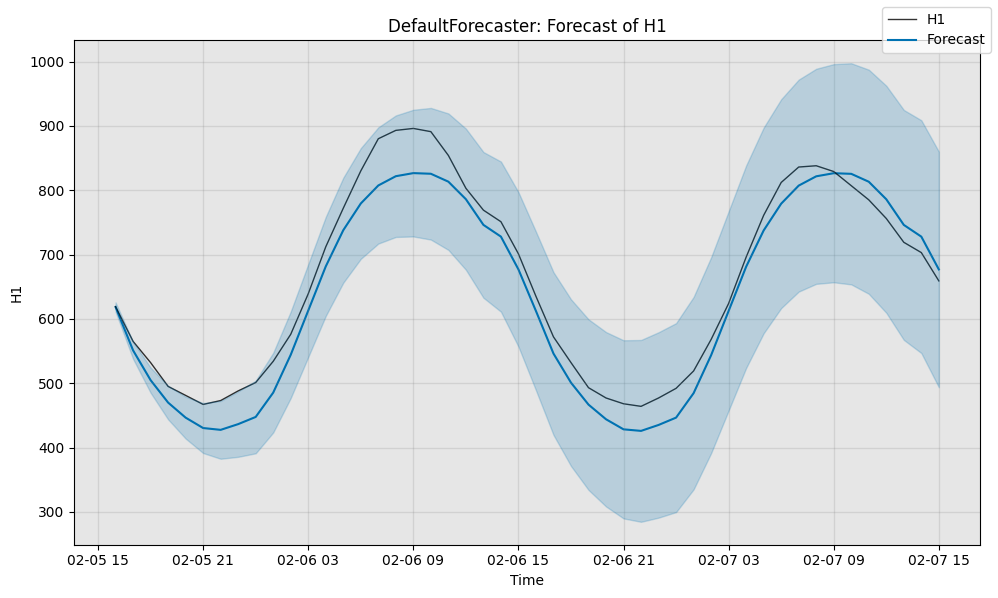
最后，我们对模型进行定量评估。sMAPE用于衡量预测误差，范围为0到100（越低越好），而MSIS用于评估95%置信区间的质量，范围同样为0到100（越低越好）。

sMAPE（Symmetric Mean Absolute Percentage Error，对称平均绝对百分比误差 和 MSIS（Mean Scaled Interval Score，均值尺度区间得分是两种常用的时间序列预测误差评估指标。

1. sMAPE（对称平均绝对百分比误差）

sMAPE是一种衡量预测值与实际值误差的指标，特别适用于时间序列预测。它的计算方式与常见的MAPE（平均绝对百分比误差）类似，但进行了对称处理，使得它对高估和低估的惩罚更加平衡。

sMAPE的公式如下：

$\text{sMAPE} = \frac{1}{n} \sum_{i=1}^{n} \frac{|y_i - \hat{y_i}|}{\frac{|y_i| + |\hat{y_i}|}{2}} \times 100\%$

$y_i$ 是实际值
$\hat{y_i}$ 是预测值
$n$ 是数据点的数量

解释：

sMAPE的取值范围为0到100，数值越小，表示预测误差越小，模型效果越好。
sMAPE在实际值和预测值接近0时表现更稳定，相对于MAPE对异常值的敏感性更低。

2. MSIS（均值尺度区间得分）

MSIS用于评估预测模型生成的预测区间（如95%置信区间）的质量，既考虑区间的宽度，也考虑实际值是否落在区间内。它衡量了预测区间的准确性和覆盖率，主要用于间隔预测的场景。

MSIS的计算公式为：

$\text{MSIS} = \frac{1}{n} \sum_{i=1}^{n} \left[ U_i - L_i + \frac{2}{\alpha} (L_i - y_i) \cdot 1(y_i < L_i) + \frac{2}{\alpha} (y_i - U_i) \cdot 1(y_i > U_i) \right]$

$L_i$ 和 $U_i$ 是第 $i$ 个时间点的预测下界和上界（置信区间）
$y_i$ 是实际值
$1(\cdot)$ 是指示函数，若条件为真则值为1，否则为0
$\alpha$ 是置信区间的显著性水平（如95%置信区间对应 $\alpha = 0.05$ ）

解释：

MSIS考虑了区间宽度和预测的覆盖率，得分越低，表示预测区间的表现越好。
它不仅考虑区间的紧凑性（宽度），还惩罚那些实际值超出预测区间的情况。

这两者结合使用时，sMAPE评估预测点的准确性，MSIS评估预测区间的可靠性，能更全面地衡量预测模型的表现。

python">from scipy.stats import norm
from merlion.evaluate.forecast import ForecastMetric# Compute the sMAPE of the predictions (0 to 100, smaller is better)
smape = ForecastMetric.sMAPE.value(ground_truth=test_data, predict=test_pred)# Compute the MSIS of the model's 95% confidence interval (0 to 100, smaller is better)
lb = TimeSeries.from_pd(test_pred.to_pd() + norm.ppf(0.025) * test_err.to_pd().values)
ub = TimeSeries.from_pd(test_pred.to_pd() + norm.ppf(0.975) * test_err.to_pd().values)
msis = ForecastMetric.MSIS.value(ground_truth=test_data, predict=test_pred,insample=train_data, lb=lb, ub=ub)
print(f"sMAPE: {smape:.4f}, MSIS: {msis:.4f}")

sMAPE: 5.3424, MSIS: 19.2706

2 单变量 时间序列 预测

本笔记将指导您使用Merlion中预测器的所有关键功能。具体来说，我们将解释：

初始化预测模型（包括集成模型和自动模型选择器）
训练模型
使用模型生成预测
可视化模型的预测结果
定量评估模型
保存和加载训练好的模型
使用ForecastEvaluator模拟模型的实时部署

我们将在整个笔记中使用一个示例时间序列。现在开始加载它：

python">import matplotlib.pyplot as plt
import numpy as npfrom merlion.utils.time_series import TimeSeries
from ts_datasets.forecast import M4# Load the time series
# time_series is a time-indexed pandas.DataFrame
# trainval is a time-indexed pandas.Series indicating whether each timestamp is for training or testing
time_series, metadata = M4(subset="Hourly")[5]
trainval = metadata["trainval"]# Is there any missing data?
timedeltas = np.diff(time_series.index) # 计算时间戳之间的差值。这会返回一个数组，其中每个元素表示相邻时间戳之间的差（即时间间隔）
# 检查每个时间间隔是否与第一个时间间隔（timedeltas[0]）相等。 any函数只要有一个True，就会返回True
print(f"Has missing data: {any(timedeltas != timedeltas[0])}")# Visualize the time series and draw a dotted line to indicate the train/test split
fig = plt.figure(figsize=(10, 6))
ax = fig.add_subplot(111)
ax.plot(time_series)
ax.axvline(time_series[trainval].index[-1], ls="--", lw="2", c="k") # 在训练集的最后一个时间戳添加一条垂直线
plt.show()# Split the time series into train/test splits, and convert it to Merlion format
train_data = TimeSeries.from_pd(time_series[trainval])
test_data = TimeSeries.from_pd(time_series[~trainval])
print(f"{len(train_data)} points in train split, "f"{len(test_data)} points in test split.")

Has missing data: False

output_9_2

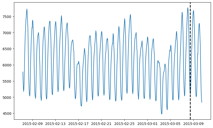
700 points in train split, 48 points in test split.

2.1 模型初始化

在本笔记中，我们将使用三种不同的预测模型：

ARIMA（经典的随机过程模型）
Prophet（Facebook 的流行时间序列预测模型）
MSES（多尺度指数平滑模型，由内部开发）

让我们先初始化每个模型。

注意： 下面代码可能会报这个错误：AttributeError: 'Prophet' object has no attribute 'stan_backend'。只需安装conda install -c conda-forge cmdstan即可解决。

python"># 导入模型和配置
from merlion.models.forecast.arima import Arima, ArimaConfig
from merlion.models.forecast.prophet import Prophet, ProphetConfig
from merlion.models.forecast.smoother import MSES, MSESConfig# 导入数据预处理变换
from merlion.transform.base import Identity
from merlion.transform.resample import TemporalResample# 所有模型的初始化使用语法 ModelClass(config)，
# 其中 config 是特定于模型的配置对象。这里是指定任何算法特定的超参数以及任何数据预处理变换的地方。# ARIMA 假设输入数据在均匀间隔下进行采样，因此我们将其变换设置为在均匀间隔下进行采样。我们还必须指定最大预测范围。
config1 = ArimaConfig(max_forecast_steps=100, order=(20, 1, 5), # ARIMA 模型的超参数transform=TemporalResample(granularity="1h"))
model1 = Arima(config1)# Prophet 对输入数据没有实际假设（并且不需要最大预测范围），因此我们通过使用Identity 变换跳过数据预处理。
config2 = ProphetConfig(max_forecast_steps=None, transform=Identity())
model2 = Prophet(config2)# MSES 假设输入数据在规则间隔下采样，并要求我们指定最大预测范围。我们还将在这里指定其回溯超参数为 60。
config3 = MSESConfig(max_forecast_steps=100, max_backstep=60, # 模型在计算时回溯查看前60步历史数据，以进行平滑和预测。transform=TemporalResample(granularity="1h"))
model3 = MSES(config3)

现在我们已经初始化了各个单独的模型，我们还将它们组合成两种不同的集成模型：集成模型简单地取每个单独模型预测结果的平均值，而选择器则根据其 sMAPE（对称平均绝对百分比误差）选择表现最好的单独模型。sMAPE 是一种用于评估连续预测质量的指标。计算公式见上。

python">from merlion.evaluate.forecast import ForecastMetric
from merlion.models.ensemble.combine import Mean, ModelSelector
from merlion.models.ensemble.forecast import ForecasterEnsemble, ForecasterEnsembleConfig# ForecasterEnsemble 是一个预测器，we treat it as a first-class model.
# 它的配置文件接受一个组合器对象，用于指定如何组合集成中各个模型的预测结果。
# 下面我们介绍两种指定集成实际模型的方法。# 第一种方式是在初始化 ForecasterEnsembleConfig 时提供集成中的模型。
#
# 这里的组合器将简单地取集成中各个模型预测结果的平均值
ensemble_config = ForecasterEnsembleConfig(combiner=Mean(), models=[model1, model2, model3])
ensemble = ForecasterEnsemble(config=ensemble_config)# 或者，可以在直接初始化 ForecasterEnsemble 时指定模型。
#
# 这里的组合器使用 sMAPE 来比较各个模型，并选择 sMAPE 最低的模型
selector_config = ForecasterEnsembleConfig(combiner=ModelSelector(metric=ForecastMetric.sMAPE))
selector = ForecasterEnsemble(config=selector_config, models=[model1, model2, model3])

2.2 训练模型

所有的预测模型（以及集成模型）共享相同的训练 API。train() 方法返回模型在训练数据上的预测结果和这些预测结果的标准误差。请注意，如果模型不支持不确定性估计（例如 MSES 和集成模型），标准误差将为 None。

python">print(f"Training {type(model1).__name__}...")
forecast1, stderr1 = model1.train(train_data)print(f"\nTraining {type(model2).__name__}...")
forecast2, stderr2 = model2.train(train_data)print(f"\nTraining {type(model3).__name__}...")
forecast3, stderr3 = model3.train(train_data)print("\nTraining ensemble...")
forecast_e, stderr_e = ensemble.train(train_data)print("\nTraining model selector...")
forecast_s, stderr_s = selector.train(train_data)print("Done!")

ForecastEvaluator: 100%|██████████| 500400/500400 [00:00<00:00, 3322678.56it/s]
20:12:21 - cmdstanpy - INFO - Chain [1] start processing
20:12:21 - cmdstanpy - INFO - Chain [1] done processing
ForecastEvaluator: 100%|██████████| 500400/500400 [00:00<00:00, 5176148.13it/s]
ForecastEvaluator: 100%|██████████| 500400/500400 [00:00<00:00, 704073.97it/s] 
Done!

2.3 模型推断

要从训练好的模型中获取预测结果，我们只需调用 model.forecast() 方法，并传入希望模型生成预测的 Unix 时间戳。在许多情况下，您可以直接从时间序列中获取这些时间戳，如下所示。

python"># Truncate the test data to ensure that we are within each model's maximum
# forecast horizon.
sub_test_data = test_data[:50]# Obtain the time stamps corresponding to the test data
time_stamps = sub_test_data.univariates[sub_test_data.names[0]].time_stamps# Get the forecast & standard error of each model. These are both
# merlion.utils.TimeSeries objects. Note that the standard error is None for
# models which don't support uncertainty estimation (like MSES and all
# ensembles).
forecast1, stderr1 = model1.forecast(time_stamps=time_stamps)
forecast2, stderr2 = model2.forecast(time_stamps=time_stamps)# 您可以选择性地指定一个时间序列前缀作为上下文。如果没有指定，
# 前缀默认是训练数据。这里我们只是明确表达了这种依赖关系。
# 更广泛地说，如果您希望使用预训练模型对训练结束后的未来数据进行预测，该功能将非常有用。
forecast3, stderr3 = model3.forecast(time_stamps=time_stamps, time_series_prev=train_data)# The same options are available for ensembles as well, though the stderr is None
forecast_e, stderr_e = ensemble.forecast(time_stamps=time_stamps)
forecast_s, stderr_s = selector.forecast(time_stamps=time_stamps, time_series_prev=train_data)

2.4 模型可视化和定量评估

可视化模型的预测结果并使用标准指标（如 sMAPE）进行定量评估是相对直观的。我们在下面展示了五个模型的示例。

接下来，我们使用 sMAPE 指标对模型进行定量评估。不过，ForecastMetric 还包括许多其他选项。一般情况下，您可以使用以下语法进行评估：

ForecastMetric.<metric_name>.value(ground_truth=ground_truth, predict=forecast)

其中，<metric_name> 是评估指标的名称（有关详细信息和更多选项，请参见 API 文档），ground_truth 是原始时间序列，forecast 是模型返回的预测结果。我们在下面展示了使用 ForecastMetric.sMAPE 的具体示例。

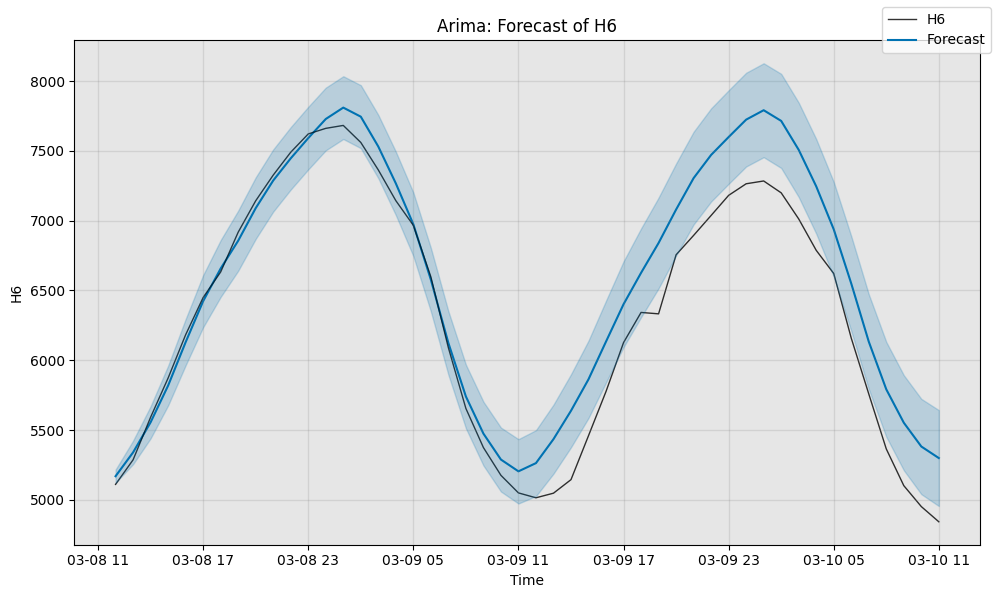
python">from merlion.evaluate.forecast import ForecastMetric# We begin by computing the sMAPE of ARIMA's forecast (scale is 0 to 100)
smape1 = ForecastMetric.sMAPE.value(ground_truth=sub_test_data,predict=forecast1)
print(f"{type(model1).__name__} sMAPE is {smape1:.3f}")# Next, we can visualize the actual forecast, and understand why it
# attains this particular sMAPE. Since ARIMA supports uncertainty
# estimation, we plot its error bars too.
fig, ax = model1.plot_forecast(time_series=sub_test_data,plot_forecast_uncertainty=True)
plt.show()

Arima sMAPE is 3.827

output_19_1

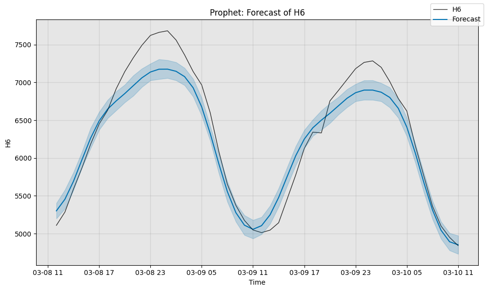
python"># We begin by computing the sMAPE of Prophet's forecast (scale is 0 to 100)
smape2 = ForecastMetric.sMAPE.value(sub_test_data, forecast2)
print(f"{type(model2).__name__} sMAPE is {smape2:.3f}")# Next, we can visualize the actual forecast, and understand why it
# attains this particular sMAPE. Since Prophet supports uncertainty
# estimation, we plot its error bars too.
# 请注意，我们也可以在这里指定 time_series_prev，但除非我们同时提供关键字参数 plot_time_series_prev=True，否则它不会被可视化。
fig, ax = model2.plot_forecast(time_series=sub_test_data,time_series_prev=train_data,plot_forecast_uncertainty=True)
plt.show()

Prophet sMAPE is 3.120

output_20_1

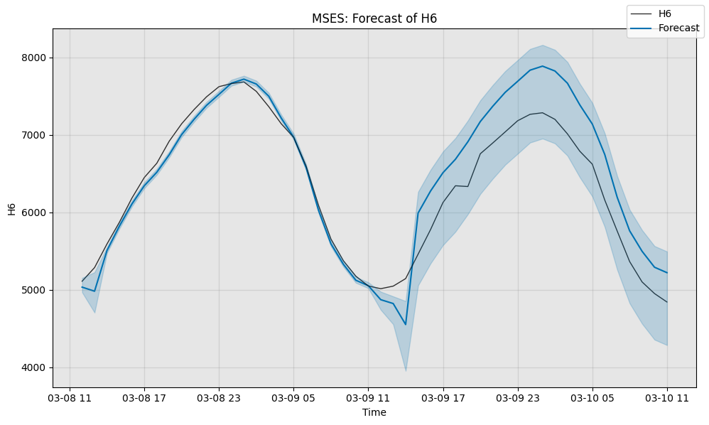
python"># We begin by computing the sMAPE of MSES's forecast (scale is 0 to 100)
smape3 = ForecastMetric.sMAPE.value(sub_test_data, forecast3)
print(f"{type(model3).__name__} sMAPE is {smape3:.3f}")# Next, we visualize the actual forecast, and understand why it
# attains this particular sMAPE.
fig, ax = model3.plot_forecast(time_series=sub_test_data,plot_forecast_uncertainty=True)
plt.show()

MSES sMAPE is 4.377

output_21_1

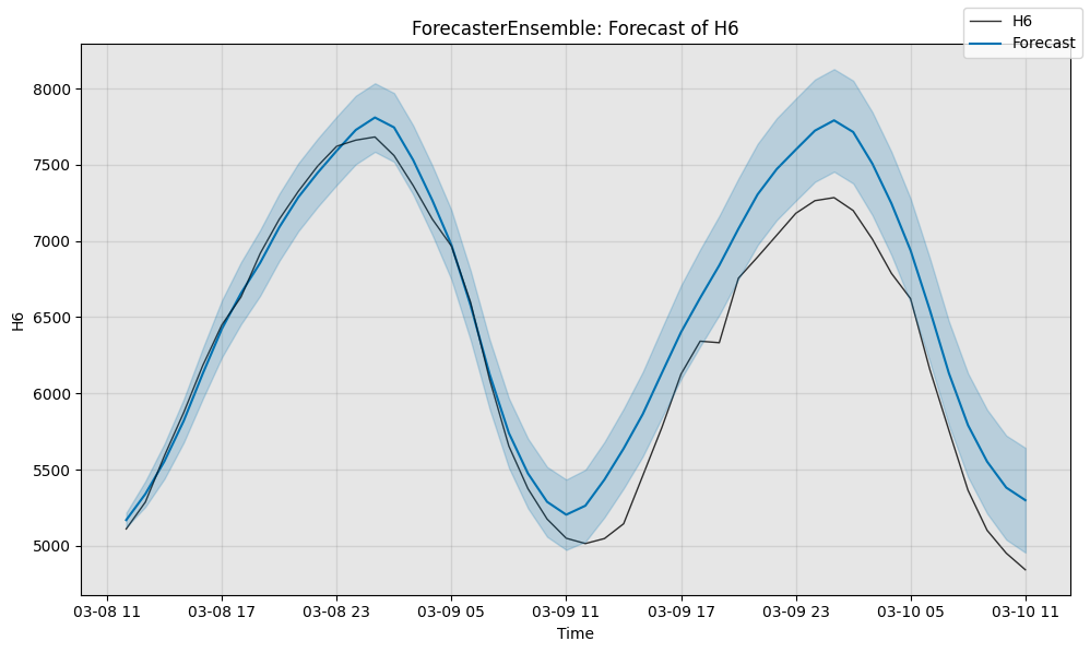
python"># Compute the sMAPE of the ensemble's forecast (scale is 0 to 100)
smape_e = ForecastMetric.sMAPE.value(sub_test_data, forecast_e)
print(f"Ensemble sMAPE is {smape_e:.3f}")# Visualize the forecast.
fig, ax = ensemble.plot_forecast(time_series=sub_test_data,plot_forecast_uncertainty=True)
plt.show()

Ensemble sMAPE is 2.506

output_22_1

python"># Compute the sMAPE of the selector's forecast (scale is 0 to 100)
smape_s = ForecastMetric.sMAPE.value(sub_test_data, forecast_s)
print(f"Selector sMAPE is {smape_s:.3f}")# Visualize the forecast.
fig, ax = selector.plot_forecast(time_series=sub_test_data,plot_forecast_uncertainty=True)
plt.show()

Selector sMAPE is 3.827

output_23_1

2.5 保存和加载模型

所有模型都有 save() 方法和 load() 类方法。模型也可以借助 ModelFactory 进行加载，其适用于任意模型。save() 方法会在指定路径下创建一个新目录，在该目录中保存一个表示模型配置的 JSON 文件，以及一个用于模型状态的二进制文件。

这里以 Prophet 模型（model2）为例来演示这些行为。

python">import json
import os
import pprint
from merlion.models.factory import ModelFactory# Save the model
os.makedirs("models", exist_ok=True) # 目录不存在则创建，存在则不报错
path = os.path.join("models", "prophet")
model2.save(path)# Print the config saved
pp = pprint.PrettyPrinter()
with open(os.path.join(path, "config.json")) as f:print(f"{type(model2).__name__} Config")pp.pprint(json.load(f))# Load the model using Prophet.load()
model2_loaded = Prophet.load(dirname=path)# Load the model using the ModelFactory
model2_factory_loaded = ModelFactory.load(name="Prophet", model_path=path)

Prophet Config
{'daily_seasonality': 'auto','dim': 1,'exog_aggregation_policy': 'Mean','exog_missing_value_policy': 'ZFill','exog_transform': {'bias': None,'name': 'MeanVarNormalize','normalize_bias': True,'normalize_scale': True,'scale': None},'holidays': None,'invert_transform': True,'max_forecast_steps': None,'seasonality_mode': 'additive','target_seq_index': 0,'transform': {'name': 'Identity'},'uncertainty_samples': 100,'weekly_seasonality': 'auto','yearly_seasonality': 'auto'}

我们可以对集成模型做完全相同的操作！请注意，集成模型会将其基础模型存储在一个嵌套结构中。此外，组合器（保存在 ForecasterEnsembleConfig 中）会跟踪每个模型所达到的 sMAPE 值（metric_values 键）。所有这些信息都反映在配置中。

python"># Save the selector
path = os.path.join("models", "selector")
selector.save(path)# Print the config saved. Note that we've saved all individual models,
# and their paths are specified under the model_paths key.
pp = pprint.PrettyPrinter()
with open(os.path.join(path, "config.json")) as f:print(f"Selector Config")pp.pprint(json.load(f))# Load the selector
selector_loaded = ForecasterEnsemble.load(dirname=path)# Load the selector using the ModelFactory
selector_factory_loaded = ModelFactory.load(name="ForecasterEnsemble", model_path=path)

Selector Config
{'combiner': {'_override_models_used': {},'abs_score': False,'metric': 'ForecastMetric.sMAPE','metric_values': [4.92497231969932,7.115701089329411,14.33041679538694],'n_models': 3,'name': 'ModelSelector'},'dim': 1,'exog_aggregation_policy': 'Mean','exog_missing_value_policy': 'ZFill','exog_transform': {'bias': None,'name': 'MeanVarNormalize','normalize_bias': True,'normalize_scale': True,'scale': None},'invert_transform': True,'max_forecast_steps': None,'models': [{'dim': 1,'exog_aggregation_policy': 'Mean','exog_missing_value_policy': 'ZFill','exog_transform': {'bias': None,'name': 'MeanVarNormalize','normalize_bias': True,'normalize_scale': True,'scale': None},'invert_transform': True,'max_forecast_steps': 100,'name': 'Arima','order': [20, 1, 5],'target_seq_index': 0,'transform': {'aggregation_policy': 'Mean','granularity': 3600.0,'missing_value_policy': 'Interpolate','name': 'TemporalResample','origin': 1423296000.0,'remove_non_overlapping': True,'trainable_granularity': False}},{'daily_seasonality': 'auto','dim': 1,'exog_aggregation_policy': 'Mean','exog_missing_value_policy': 'ZFill','exog_transform': {'bias': None,'name': 'MeanVarNormalize','normalize_bias': True,'normalize_scale': True,'scale': None},'holidays': None,'invert_transform': True,'max_forecast_steps': None,'name': 'Prophet','seasonality_mode': 'additive','target_seq_index': 0,'transform': {'name': 'Identity'},'uncertainty_samples': 100,'weekly_seasonality': 'auto','yearly_seasonality': 'auto'},{'accel_weight': 1.0,'dim': 1,'eta': 0.0,'inflation': 1.0,'invert_transform': True,'max_backstep': 60,'max_forecast_steps': 100,'name': 'MSES','optimize_acc': True,'phi': 2.0,'recency_weight': 0.5,'rho': 0.0,'target_seq_index': 0,'transform': {'aggregation_policy': 'Mean','granularity': 3600.0,'missing_value_policy': 'Interpolate','name': 'TemporalResample','origin': 1423296000.0,'remove_non_overlapping': True,'trainable_granularity': False}}],'target_seq_index': 0,'transform': {'name': 'Identity'},'verbose': False}

2.6 模拟实时模型部署

典型的模型部署场景如下：

在一些最近的历史数据上训练初始模型。
在规则的时间间隔内，获取模型的某个预测范围的预测结果。
在规则的重训练频率（retrain_freq）内，使用最近的数据重新训练整个模型。
可选地，指定模型在训练时应使用的最大数据量（train_window）。

我们提供了一个 ForecastEvaluator 对象，用于模拟上述部署场景，并允许用户根据所选的评估指标评估预测器的质量。我们在下面展示两个示例，第一个示例使用 ARIMA，第二个示例使用模型 selector。

创建一个 ForecastEvaluator 对象，该对象用于评估时间序列预测模型的性能。以下是对每个参数的详细解释：

model=model:
- 这里的 model 是你之前定义或初始化的时间序列预测模型。通过将其传递给 ForecastEvaluator，评估器将能够使用这个模型来生成预测。
config=ForecastEvaluatorConfig(...):
- 这部分是用来配置评估器的参数，具体如下：
- cadence="1h":
  - 表示每小时获取一次模型的预测。即，评估器将在每小时的时间点上运行模型，生成预测。
- horizon="6h":
  - 表示模型将预测未来6小时的值。这意味着在每个小时的预测中，模型将给出接下来的6小时的预期值。
- retrain_freq="12h":
  - 表示模型将每12小时重新训练一次。这是为了确保模型能够适应新的数据和趋势，保持预测的准确性。
- train_window="14d":
  - 指定模型在重新训练时将使用过去14天的数据。这意味着当模型被重新训练时，它只会利用最近两周的数据，以减少过时数据的影响并集中在最新的趋势上。

这段代码通过配置评估器，设置了预测的频率、范围和模型的重新训练策略，从而使得模型的评估过程更加灵活和高效。

python">from merlion.evaluate.forecast import ForecastEvaluator, ForecastEvaluatorConfig, ForecastMetricdef create_evaluator(model):# 重新初始化模型，以便我们可以从头开始重新训练它model.reset()# 为模型创建评估管道，其中我们# -- 每小时获取一次模型的预测# -- 让模型预测6小时的范围# -- 每12小时重新训练模型# -- 当我们重新训练模型时，仅使用过去2周的数据进行训练evaluator = ForecastEvaluator(model=model, config=ForecastEvaluatorConfig(cadence="1h", horizon="6h", retrain_freq="12h", train_window="14d"))return evaluator

首先，让我们评估 ARIMA 模型。

python"># Obtain the results of running the evaluation pipeline for ARIMA.
# These result objects are to be treated as a black box, and should be
# passed directly to the evaluator's evaluate() method.
model1_evaluator = create_evaluator(model1)
model1_train_result, model1_test_result = model1_evaluator.get_predict(train_vals=train_data, test_vals=test_data)

ForecastEvaluator: 100%|██████████| 169200/169200 [00:16<00:00, 16676.23it/s]d:\ANACONDA\envs\merlion\lib\site-packages\merlion\models\forecast\sarima.py:131: FutureWarning: Series.__getitem__ treating keys as positions is deprecated. In a future version, integer keys will always be treated as labels (consistent with DataFrame behavior). To access a value by position, use `ser.iloc[pos]`last_val = val_prev[-1]
ForecastEvaluator: 100%|██████████| 169200/169200 [00:16<00:00, 10298.87it/s]

python"># Evaluate ARIMA's sMAPE and RMSE
smape = model1_evaluator.evaluate(ground_truth=test_data,predict=model1_test_result,metric=ForecastMetric.sMAPE)
rmse  = model1_evaluator.evaluate(ground_truth=test_data,predict=model1_test_result,metric=ForecastMetric.RMSE)
print(f"{type(model1).__name__} sMAPE: {smape:.3f}")
print(f"{type(model1).__name__} RMSE:  {rmse:.3f}")

Arima sMAPE: 2.016
Arima RMSE:  143.490

接下来，我们将评估集成模型（在每次调用模型时，取 ARIMA、Prophet 和 MSES 的平均预测值）。

python"># Obtain the results of running the evaluation pipeline for the ensemble.
# These result objects are to be treated as a black box, and should be
# passed directly to the evaluator's evaluate() method.
ensemble_evaluator = create_evaluator(ensemble)
ensemble_train_result, ensemble_test_result = ensemble_evaluator.get_predict(train_vals=train_data, test_vals=test_data)

ForecastEvaluator: 100%|██████████| 169200/169200 [00:32<00:00, 11233.26it/s]d:\ANACONDA\envs\merlion\lib\site-packages\merlion\models\forecast\sarima.py:131: FutureWarning: Series.__getitem__ treating keys as positions is deprecated. In a future version, integer keys will always be treated as labels (consistent with DataFrame behavior). To access a value by position, use `ser.iloc[pos]`last_val = val_prev[-1]
ForecastEvaluator: 100%|██████████| 169200/169200 [00:32<00:00, 5246.34it/s]

python"># Evaluate the selector's sMAPE and RMSE
smape = ensemble_evaluator.evaluate(ground_truth=test_data,predict=ensemble_test_result,metric=ForecastMetric.sMAPE)
rmse  = ensemble_evaluator.evaluate(ground_truth=test_data,predict=ensemble_test_result,metric=ForecastMetric.RMSE)
print(f"Ensemble sMAPE: {smape:.3f}")
print(f"Ensemble RMSE:  {rmse:.3f}")

Ensemble sMAPE: 2.909
Ensemble RMSE:  211.509