一、概述

上一篇文章《自然语言处理入门1——单词的表示和距离》我们谈到了单词的表示以及距离的相似度计算，从而可以预测哪个单词的出现概率最高，这种方法被成为基于计数的方法，因为从根本上都要计算单词的出现次数，构建共现矩阵。不过这种方法有个问题，就是计算量太大，特别是现实当中的语料库都很大，一本小说可能就有几十万上百万字，构建100万x100万的共现矩阵的开销是不可接受的，特别是还要在上面做SVD计算。所以引入了神经网络，也被称作基于推理的方法。基于计数的方法需要一次性学习所有数据，而神经网络可以用小批量的数据进行部分学习，不断改进，即使语料库很大也可以进行学习。（对应《深度学习进阶：自然语言处理》的第三章）

二、CBOW模型

我们考虑一种最简单的情况，基于上下文预测出中间缺失的单词，并且仅仅预测中间缺失的一个单词，上下文也只用一个单词，如“ you ? goodbye and i say hello.”，用you和googdbye去预测问号的值。这种预测就类似于完形填空，是比较简单的一种情况。处理这种完形填空问题的一个代表模型是CBOW。CBOW是根据上下文预测目标词的神经网络，这里的目标词是指中间的单词，如例子中的问号处，上下文就是指周围的单词。通过训练这个模型，我们可以使其尽可能正确的预测出中间缺少的单词。

书中给出的CBOW的模型结构图如下：

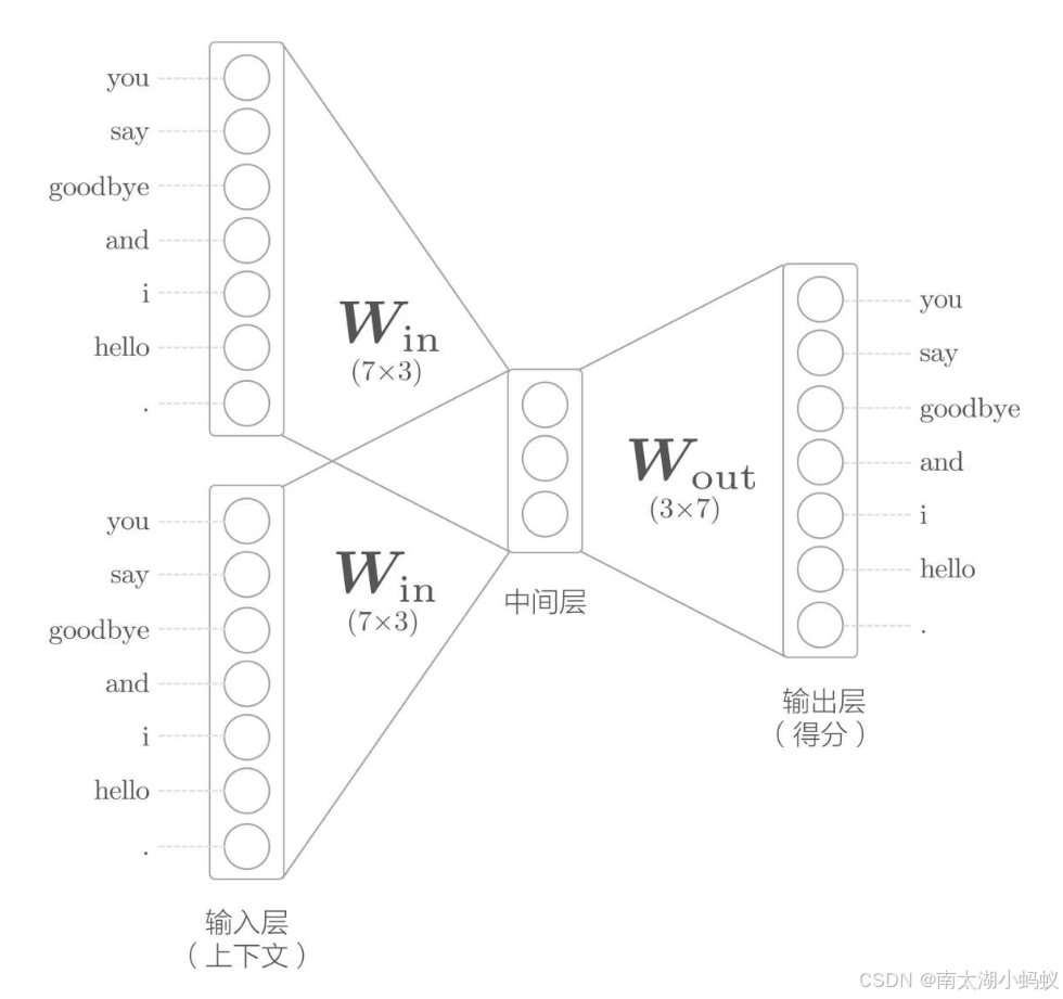
其实就是输入待预测目标周围的两个单词作为上下文，和中间层做一个全连接，再和输出层做一个全连接得到分数。其中输入和输出都用one-hot表示法表示。下图表示的更为清晰：

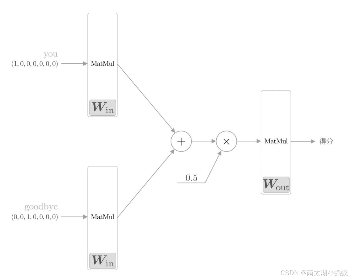
流程如下：

1）将上下文输入表示成one-hot形式，随机生成一个输入权重矩阵和输出权重矩阵；

2）两个输入分别乘以输入权重矩阵，注意两个输入都乘以同一个权重矩阵；

3）把得到的两个结果相加后除以2，得到中间结果；

4）把中间结果乘以输出权重矩阵，得到分数；

5）把得分进行softmax处理，转化成概率，得到最大的预测值；

6）把预测值和目标值进行比较，求得交叉熵；

7）进行误差反向传播，更新权重矩阵；

8）重复上面的步骤，直到模型输出的值和真实值足够接近，停止。

这里，我们不断训练，调整的就是两个权重矩阵，直到用这两个权重矩阵可以准确的完成“完形填空”。这里我和书上不一样的地方在于，我的目标不是获取单词的向量表示，而且根据上下文来预测单词，所以书中模型训练后没有考虑预测的问题，我把预测部分实现了一下。下面我们具体来看程序。

三、代码实现

根据之前的流程，首先要把语料库中单词表示成one-hot形式。我们需要先构建上下文和目标单词的向量表示。

python">import numpy as nptext = 'You say goodbye and I say hello.'
corpus, word_to_id, id_to_word = preprocess(text)
print(corpus)
print(id_to_word)
# 输出：
[0 1 2 3 4 1 5 6]
{0: 'you', 1: 'say', 2: 'goodbye', 3: 'and', 4: 'i', 5: 'hello', 6: '.'}

python"># 构建上下文和目标向量
def create_contexts_target(corpus, window_size=1):target = corpus[window_size:-window_size]contexts = []for idx in range(window_size, len(corpus)-window_size):#print("idx=======",idx)cs = []for t in range(-window_size, window_size+1):if t==0:continuecs.append(corpus[idx+t])contexts.append(cs)return np.array(contexts), np.array(target)contexts, target = create_contexts_target(corpus)
print(contexts)
print(target)
# 输出：
[[0 2][1 3][2 4][3 1][4 5][1 6]]
[1 2 3 4 1 5]

接下来，我们用一个函数把数字表示转换成one-hot表示：

python"># 将上下文和目标词转换成one-hot表示
def convert_one_hot(corpus, vocab_size):'''转换为one-hot表示:param corpus: 单词ID列表（一维或二维的NumPy数组）:param vocab_size: 词汇个数:return: one-hot表示（二维或三维的NumPy数组）'''N = corpus.shape[0]if corpus.ndim == 1:one_hot = np.zeros((N, vocab_size), dtype=np.int32)for idx, word_id in enumerate(corpus):one_hot[idx, word_id] = 1elif corpus.ndim == 2:C = corpus.shape[1]one_hot = np.zeros((N, C, vocab_size), dtype=np.int32)for idx_0, word_ids in enumerate(corpus):for idx_1, word_id in enumerate(word_ids):one_hot[idx_0, idx_1, word_id] = 1return one_hotvocab_size = len(word_to_id)
target = convert_one_hot(target, vocab_size)
contexts = convert_one_hot(contexts, vocab_size)
print(target)
print(contexts)
# 输出：
[[0 1 0 0 0 0 0][0 0 1 0 0 0 0][0 0 0 1 0 0 0][0 0 0 0 1 0 0][0 1 0 0 0 0 0][0 0 0 0 0 1 0]]
[[[1 0 0 0 0 0 0][0 0 1 0 0 0 0]][[0 1 0 0 0 0 0][0 0 0 1 0 0 0]][[0 0 1 0 0 0 0][0 0 0 0 1 0 0]][[0 0 0 1 0 0 0][0 1 0 0 0 0 0]][[0 0 0 0 1 0 0][0 0 0 0 0 1 0]][[0 1 0 0 0 0 0][0 0 0 0 0 0 1]]]

可以看到，我们把词向量都表示成了one-hot格式的数据。接下来，我们定义模型。

python"># 矩阵乘法模块
class MatMul:def __init__(self, W):self.params = [W]self.grads = [np.zeros_like(W)]self.x = Nonedef forward(self, x):W, = self.paramsout = np.dot(x, W)self.x = xreturn outdef backward(self, dout):W, = self.paramsdx = np.dot(dout, W.T)dW = np.dot(self.x.T, dout)self.grads[0][...] = dWreturn dx# 实现CBOW类
class SimpleCBOW:def __init__(self, vocab_size, hidden_size):V,H = vocab_size, hidden_size# 初始化权重W_in = 0.01*np.random.randn(V,H).astype('f')W_out = 0.01*np.random.randn(H,V).astype('f')# 生成层self.in_layer0 = MatMul(W_in)self.in_layer1 = MatMul(W_in)self.out_layer = MatMul(W_out)self.loss_layer = SoftmaxWithLoss()layers = [self.in_layer0,self.in_layer1,self.out_layer]self.params, self.grads = [], []for layer in layers:self.params += layer.paramsself.grads += layer.gradsdef forward(self, contexts, target):print("contexts[:,0].shape: ",contexts[:,0].shape)h0 = self.in_layer0.forward(contexts[:,0])h1 = self.in_layer1.forward(contexts[:,1])h = (h0 + h1) * 0.5score = self.out_layer.forward(h)loss = self.loss_layer.forward(score, target)return lossdef backward(self, dout=1):ds = self.loss_layer.backward(dout)da = self.out_layer.backward(ds)da *= 0.5self.in_layer0.backward(da)self.in_layer1.backward(da)return Nonedef get_params(self): # 获取各层训练后的参数return self.in_layer0,self.in_layer1,self.out_layer

下面我们再定义一个训练函数：

python">import numpy
import time
import matplotlib.pyplot as plt
class Trainer:def __init__(self, model, optimizer):self.model = modelself.optimizer = optimizerself.loss_list = []self.eval_interval = Noneself.current_epoch = 0def fit(self, x, t, max_epoch=10, batch_size=32, max_grad=None, eval_interval=20):print("x.shape: ",x.shape)data_size = len(x)print("data_size: ",data_size)max_iters = data_size // batch_sizeprint("max_iters: ",max_iters)self.eval_interval = eval_intervalmodel, optimizer = self.model, self.optimizertotal_loss = 0loss_count = 0start_time = time.time()for epoch in range(max_epoch):# 打乱idx = numpy.random.permutation(numpy.arange(data_size))x = x[idx]t = t[idx]print("x.shape:+++++++++", x.shape)for iters in range(max_iters):batch_x = x[iters*batch_size:(iters+1)*batch_size]batch_t = t[iters*batch_size:(iters+1)*batch_size]print("batch_x.shape: ",batch_x.shape)# 计算梯度，更新参数loss = model.forward(batch_x, batch_t)model.backward()# 将共享的权重整合为1个params, grads = remove_duplicate(model.params, model.grads)  if max_grad is not None:clip_grads(grads, max_grad)optimizer.update(params, grads)total_loss += lossloss_count += 1# 评价if (eval_interval is not None) and (iters % eval_interval) == 0:avg_loss = total_loss / loss_countelapsed_time = time.time() - start_timeprint('| epoch %d |  iter %d / %d | time %d[s] | loss %.2f'% (self.current_epoch + 1, iters + 1, max_iters, elapsed_time, avg_loss))self.loss_list.append(float(avg_loss))total_loss, loss_count = 0, 0self.current_epoch += 1# 画出训练过程中损失值的变化def plot(self, ylim=None):x = numpy.arange(len(self.loss_list))if ylim is not None:plt.ylim(*ylim)plt.plot(x, self.loss_list, label='train')plt.xlabel('iterations (x' + str(self.eval_interval) + ')')plt.ylabel('loss')plt.show()

我们用书中给出的一句话来进行测试这个模型：

python"># 训练
window_size = 1
hidden_size = 5
batch_size = 3
max_epoch = 1000
text = 'You say goodbye and I say hello.'
corpus, word_to_id, id_to_word = preprocess(text)
contexts, target = create_contexts_target(corpus)
vocab_size = len(word_to_id)
target = convert_one_hot(target, vocab_size)
contexts = convert_one_hot(contexts, vocab_size)
print("contexts.shape: ",contexts.shape)model = SimpleCBOW(vocab_size, hidden_size)
optimizer = Adam()
trainer = Trainer(model, optimizer)
trainer.fit(contexts, target, max_epoch, batch_size)
trainer.plot()
# 输出：
contexts.shape:  (6, 2, 7)
x.shape:  (6, 2, 7)
data_size:  6
max_iters:  2
x.shape:+++++++++ (6, 2, 7)
batch_x.shape:  (3, 2, 7)
contexts[:,0].shape:  (3, 7)
| epoch 1 |  iter 1 / 2 | time 0[s] | loss 1.95
... ...

训练过程如下：

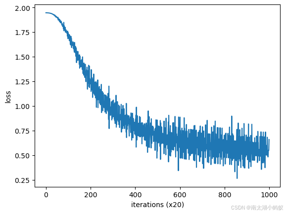
可以看到，随着训练步骤的不断迭代，损失值不断下降。我们可以获取训练后模型的权重值，根据权重值就可以进行预测了。

这里我们使用的语料库是一句话，这句话有8个单词，词向量是7个，上下文一共有六个，分别是(you,goodbye),(say,and),(goodbye,I),(and,say),(I,hello),(say,.)6种情况，每个单词进行one-hot表示后，变成(1,7)向量，每个上下文是(2,7)向量，总体的文本库大小是(6,2,7)，所以contexts.shape是（6，2，7），又由于batch_size是3，所以模型训练的时候，输入contexts是[3,2,7]，其中3是batch_size，2是前后两个上下文向量，7是词表大小。contexts[:,0]和contexts[:,1]是分别指一前一后两个上下文向量，每一个的大小都是[3,7]，之所以是[3,7]不是[1,7]是因为有三个向量同时输入作批处理。

python">in_layer0,in_layer1,out_layer = model.get_params()
vocab_size = len(word_to_id)
context1 = convert_one_hot(np.array([word_to_id['you']]), vocab_size)
context2 = convert_one_hot(np.array([word_to_id['goodbye']]), vocab_size)
print(context1.shape)
h0 = in_layer0.forward(context1)
h1 = in_layer1.forward(context2)
h = (h0+h1)*0.5
o = out_layer.forward(h)
print(o)
print(np.argmax(o))
# 输出：
(1, 7)
[[-0.85405053  3.98822799 -4.11465032  2.95836502 -4.12735609 -0.4473659-0.8498025 ]]
1

可以看到，根据you和goodbye作为上下文，预测出的单词序号是1，从word_to_id中，我们可以发现id为1的单词是say，跟我们的原文是一致的，说明训练是有用的。

下面，我们用中文来试试，和上一篇文章一样，用“小明今天去银泰双子楼看电影了”这句话作为语料库，在数据处理中，主要的区别就在于对中文语句要做一个分词从而得到单词，不能像英语一样直接切分，因为汉字的语义最小单位是词，而不是单个字。

python">import jieba
def preprocess(text):seg_list = jieba.cut(text)words = list(seg_list)word_to_id = {}id_to_word = {}for word in words:if word not in word_to_id:new_id = len(word_to_id)word_to_id[word] = new_idid_to_word[new_id] = wordcorpus = [word_to_id[w] for w in words]corpus = np.array(corpus)return corpus, word_to_id, id_to_word# 训练
window_size = 1
hidden_size = 5
batch_size = 3
max_epoch = 1000
text = '小明今天去银泰双子楼看电影了'
corpus, word_to_id, id_to_word = preprocess(text)
contexts, target = create_contexts_target(corpus)
vocab_size = len(word_to_id)
target = convert_one_hot(target, vocab_size)
contexts = convert_one_hot(contexts, vocab_size)
print("contexts.shape: ",contexts.shape)model = SimpleCBOW(vocab_size, hidden_size)
optimizer = Adam()
trainer = Trainer(model, optimizer)
trainer.fit(contexts, target, max_epoch, batch_size)
trainer.plot()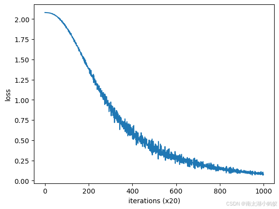

貌似中文的训练曲线还更平滑些：）下面我们也预测一下问号中的单词，“小明今天去银泰双子楼看？了”

python">print(word_to_id)
in_layer0,in_layer1,out_layer = model.get_params()
context1 = convert_one_hot(np.array([word_to_id['看']]), vocab_size)
context2 = convert_one_hot(np.array([word_to_id['了']]), vocab_size)h0 = in_layer0.forward(context1)
h1 = in_layer1.forward(context2)
h = (h0+h1)*0.5
o = out_layer.forward(h)
print(o)
print(np.argmax(o))
# 输出：
{'小明': 0, '今天': 1, '去': 2, '银泰': 3, '双子楼': 4, '看': 5, '电影': 6, '了': 7}
[[-1.63206317 -1.45593816 -2.25134312 -2.94733467  2.15194596  0.806690995.38870997 -1.62672302]]
6

根据输出，我们可以看到id为6的单词就是“电影”，也就是说这个完形填空做对了。这就是最简单的自然语言处理神经网络模型CBOW。